Semantic Security and Indistinguishability in the Quantum World

Abstract

At CRYPTO 2013, Boneh and Zhandry initiated the study of quantum-secure encryption. They proposed first indistinguishability definitions for the quantum world where the actual indistinguishability only holds for classical messages, and they provide arguments why it might be hard to achieve a stronger notion. In this work, we show that stronger notions are achievable, where the indistinguishability holds for quantum superpositions of messages. We investigate exhaustively the possibilities and subtle differences in defining such a quantum indistinguishability notion for symmetric-key encryption schemes. We justify our stronger definition by showing its equivalence to novel quantum semantic-security notions that we introduce. Furthermore, we show that our new security definitions cannot be achieved by a large class of ciphers – those which are quasi-preserving the message length. On the other hand, we provide a secure construction based on quantum-resistant pseudorandom permutations; this construction can be used as a generic transformation for turning a large class of encryption schemes into quantum indistinguishable and hence quantum semantically secure ones. Moreover, our construction is the first completely classical encryption scheme shown to be secure against an even stronger notion of indistinguishability, which was previously known to be achievable only by using quantum messages and arbitrary quantum encryption circuits.

These keywords were added by machine and not by the authors. This process is experimental and the keywords may be updated as the learning algorithm improves.

1 Introduction

Quantum computers [20] threaten many cryptographic schemes. By using Shor’s algorithm [22] and its variants [25], an adversary in possession of a quantum computer can break the security of every scheme based on factorization and discrete logarithms, including RSA, ElGamal, elliptic-curve primitives and many others. Moreover, longer keys and output lengths are required in order to maintain the security of block ciphers and hash functions [5, 12]. These difficulties led to the development of post-quantum cryptography [2], i.e., classical cryptography resistant against quantum adversaries.

When modeling the security of cryptographic schemes, care must be taken in defining exactly what property one wants to achieve. In classical security models, all parties and communications are classical. When these notions are used to prove post-quantum security, one must consider adversaries having access to a quantum computer. This means that, while the communication between the adversary and the user is still classical, the adversary might carry out computations on a quantum computer.

Such post-quantum notions of security turn out to be unsatisfying in certain scenarios. For instance, consider quantum adversaries able to use quantum superpositions of messages $\sum _x \alpha _x \mathinner {|{x}\rangle }$ instead of classical messages when communicating with the user, even though the cryptographic primitive is still classical. This kind of scenario is considered, e.g., in [4, 8, 23, 26, 28]. Such a setting might for example occur in a situation where one party using a quantum computer encrypts messages for another party that uses a classical computer and an adversary is able to observe the outcome of the quantum computation before measurement. Other examples are an attacker which is able to trick a classical device into showing quantum behavior, or a classical scheme which is used as subprotocol in a larger quantum protocol. Another possibility occurs when using obfuscation. There are applications where one might want to distribute the obfuscated code of a symmetric-key encryption scheme (with the secret key hardcoded) in order to allow a third party to generate ciphertexts without being able to retrieve the key - think of this as building public-key encryption from symmetric-key encryption using Indistinguishability Obfuscation. Because in these cases an adversary receives the classical code for producing encryptions, he could implement the code on his local quantum computer and query the resulting quantum circuit on a superposition of inputs. Moreover, even in quantum reductions for classical schemes situations could arise where superposition access is needed. A typical example are impossibility results (such as meta-reductions [7]), where giving the adversary additional power often rules out a broader range of secure reductions. Notions covering such settings are often called quantum-security notions. In this work we propose new quantum-security notions for encryption schemes.

For encryption, the notion of semantic security [10, 11] has been traditionally used. This notion models in abstract terms the fact that, without the corresponding decryption key, it is impossible not only to correctly decrypt a ciphertext, but even to recover any non-trivial information about the underlying plaintext. The exact definition of semantic security is cumbersome to work with in security proofs as it is simulation-based. Therefore, the simpler notion of ciphertext indistinguishability has been introduced. This notion is given in terms of an interactive game where an adversary has to distinguish the encryptions of two messages of his choice. The advantage of this definition is that it is easier to work with than (but equivalent to) semantic security.

To the best of our knowledge, no quantum semantic-security notions for classical encryption schemes have been proposed so far. For indistinguishability, Boneh and Zhandry introduced indistinguishability notions for quantum-secure encryption under chosen-plaintext attacks in a recent work [4]. They consider a model (IND-qCPA) where a quantum adversary can query the encrypting device in superposition during a learning phase but is limited to classical communication during the actual challenge phase. However, in the symmetric-key scenario, this approach has the following shortcoming: If we assume that an adversary can get quantum access in a learning phase, it seems unreasonable to assume that he cannot get such access when the actual message of interest is encrypted. Boneh and Zhandry showed that a seemingly natural notion of quantum indistinguishability is unachievable. In order to restore a meaningful definition, they resorted to the compromise of IND-qCPA.

Our Contributions. In this paper we achieve two main results. On the one hand, we initiate the study of semantic security in the quantum world, providing new definitions and a thorough discussion about the motivations and difficulties of modeling these notions correctly. This study is concluded by a suitable definition of quantum semantic security under chosen plaintext attacks (qSEM-qCPA). On the other hand, we extend the fundamental work initiated in [4] in finding suitable notions of indistinguishability in the quantum world. We show that the compromise that had to be reached there in order to define an achievable notion instead of a more natural one (i.e., IND-qCPA vs. fqIND-qCPA) can be overcome – although not trivially. We show how various other possible notions of quantum indistinguishability can be defined. All these security notions span a tree of possibilities which we analyze exhaustively in order to find the most suitable definition of quantum indistinguishability under chosen plaintext attacks (qIND-qCPA). We prove this notion to be achievable, strictly stronger than IND-qCPA, and equivalent to qSEM-qCPA, thereby completing an elegant framework of security notions in the quantum world, see Fig. 2 below for an overview.

Furthermore, we formally define the notion of a core function and quasi–length-preserving ciphers – encryption schemes which essentially do not increase the plaintext size, such as stream ciphers and many block ciphers including AES – and we show the impossibility of achieving our new security notion for this kind of schemes. While this impossibility might look worrying from an application perspective, we also present a transformation that turns a block cipher into an encryption scheme fulfilling our notion. This transformation also works in respect to an even stronger notion of indistinguishability in the quantum world, which was introduced in [6], and previously only known to be achievable in the setting of computational quantum encryption, that is, the scenario where all the parties have quantum computing capabilities, and encryption is performed through arbitrary quantum circuits operating on quantum data. Even if this scenario goes in a very different direction from the scope of our work, it is interesting to note that our construction is the first fully classical scheme secure even in respect to such a purely quantum notion of security.

Related Work. The idea of considering scenarios where a quantum adversary can force other parties into quantum behaviour has been first considered in [8]. Attacks exploiting classical encryptions in quantum superposition have been described in [13, 16, 17, 21]. In [4] the authors also consider the security of signature schemes where the adversary can have quantum access to a signing oracle. Quantum superposition queries have also been investigated relatively to the random oracle model [3]. Another quantum indistinguishability notion has been suggested (but not further analyzed) by Velema in [24]. Prior work has considered the security of quantum methods to encrypt classical data in the computational setting [15, 27]. In concurrent and independent work, Broadbent and Jeffery [6] introduce indistinguishability notions for the public- and secret-key encryption of quantum messages in the context of fully homomorphic quantum computation. We refer to Page 15 for a more detailed description of how their definitions relate to our framework. A more complete overview for these notions, including semantic security for quantum encryption schemes, can be found in another concurrent work [1].

2 Preliminaries

In this section, we briefly recall the classical security notions for encryption schemes secure against chosen plaintext attacks (CPA). In addition, we revisit the two existing indistinguishability notions for the quantum world. We start by introducing notation we will use throughout the paper.

We say that a function $f: \mathbb {N}\rightarrow \mathbb {R}$ is polynomially bounded iff there exists a polynomial p and a value $\bar{n} \in \mathbb {N}$ such that: for every $n\ge \bar{n}$ we have that $f(n) \le p(n)$; in this case we will just write $f = {\text {poly}\,\left( n\right) }$. We say that a function $\varepsilon : \mathbb {N}\rightarrow \mathbb {R}$ is negligible, if and only if for every polynomial p, there exists an $n_p \in \mathbb {N}$ such that $\varepsilon (n) \le \frac{1}{p(n)}$ for every $n \ge n_p$; in this case we will just write $\varepsilon = \text {negl}\left( n\right)$. In this work, we focus on secret-key encryption schemes. In all that follows we use $n\in \mathbb {N}$ as the security parameter.

Definition 2.1

(Secret-Key Encryption Scheme [10]). A secret-key encryption scheme is a triple of probabilistic polynomial-time algorithms $(\mathsf {Gen}$, $\mathsf {Enc}$, $\mathsf {Dec})$ operating on a message space $\mathcal {M}= \{0,1\}^m$ (where $m={\text {poly}\,\left( n\right) } \in \mathbb {N}$) that fulfills the following two conditions:

• 1. The key generation algorithm $\mathsf {Gen} (1^n)$ on input of security parameter n in unary outputs a bitstring k.

• 2. For all k in the range of $\mathsf {Gen} (1^n)$ and any message $x \in \mathcal {M}$, the algorithms $\mathsf {Enc}$ (encryption) and $\mathsf {Dec}$ (decryption) satisfy $\mathsf {Pr}[\mathsf {Dec} (k,\mathsf {Enc} (k,x)) = x] = 1$, where the probability is taken over the internal coin tosses of $\mathsf {Enc}$ and $\mathsf {Dec}$.

We write $\mathcal {K}$ for the range of $\mathsf {Gen} (1^n)$ (the key space) and $\mathsf {Enc} _k(x)$ for $\mathsf {Enc} (k,x)$.

2.1 Classical Security Notions: IND-CPA and SEM-CPA

We turn to security notions for encryption schemes. In this work, we will only look at the notions of indistinguishability of ciphertexts under adaptively chosen plaintext attack (IND-CPA), and semantic security under adaptively chosen plaintext attack (SEM-CPA), which are known to be equivalent (e.g., [10]).

Game-Based Definitions. In general these notions can be defined as a game between a challenger $\mathcal {C}$ and an adversary $\mathcal {A}$. First, $\mathcal {C}$ generates a legitimate key running $k\longleftarrow \mathsf {Gen} (1^n)$ which he uses throughout the game. The game starts with a first learning phase. A challenge phase follows where $\mathcal {A}$ receives a challenge. Afterwards, a second learning phase follows, and finally $\mathcal {A}$ has to output a solution. The learning phases define the type of attack, and the challenge phase the notion captured by the game. We give all our definitions by referring to this game framework and by defining a learning and a challenge phase.

The CPA Learning Phase: $\mathcal {A}$ is allowed to adaptively ask $\mathcal {C}$ for encryptions of messages of his choice. $\mathcal {C}$ answers the queries using key k. Note that this is equivalent to saying that $\mathcal {A}$ gets oracle access to an encryption oracle that was initialized with key k.

The IND Challenge Phase: $\mathcal {A}$ defines a challenge template consisting of two equal-length messages $x_0,x_1$, and sends it to $\mathcal {C}$. The challenger $\mathcal {C}$ samples a random bit $b \mathop {\longleftarrow }\limits ^{\$}\{0,1\}$ uniformly at random, and replies with the encryption $\mathsf {Enc} _k(x_b)$. $\mathcal {A}$’s goal is to guess b.

Definition 2.2

(IND-CPA). A secret-key encryption scheme is called IND-CPA secure if the success probability of any probabilistic polynomial-time adversary winning the game defined by CPA learning phases and an IND challenge phase is at most negligibly (in n) close to 1 / 2.

The SEM Challenge Phase: $\mathcal {A}$ sends $\mathcal {C}$ a challenge template $(S_m,h_m,f_m)$ consisting of a poly-sized circuit $S_m$ specifying a distribution over m-bit long plaintexts, an advise function $h_m:\{0,1\}^m\rightarrow \{0,1\}^*$, and a target function $f_m:\{0,1\}^m\rightarrow \{0,1\}^*$. The challenger $\mathcal {C}$ replies with the pair $(\mathsf {Enc} _k(x), h_m(x))$ where x is sampled according to $S_m$. $\mathcal {A}$’s challenge is to output $f_m(x)$.

In the definition of semantic security it is not required that $\mathcal {A}$’s probability of winning the game is always negligible. Instead, $\mathcal {A}$’s success probability is compared to that of a simulator $\mathcal {S}$ that plays in a reduced game: On one hand, $\mathcal {S}$  gets no learning phases. On the other hand, during the challenge phase, $\mathcal {S}$  does not receive the ciphertext but only the output of the advice function. This use of a simulator is what makes the notion hard to work with in proofs as one has to construct a simulator for every possible $\mathcal {A}$ to prove a scheme secure.

Definition 2.3

(SEM-CPA). A secret-key encryption scheme is called SEM-CPA secure if for any probabilistic polynomial-time adversary $\mathcal {A}$ there exists a probabilistic polynomial-time simulator $\mathcal {S}$ such that the challenge templates produced by $\mathcal {S}$ and $\mathcal {A}$ are identically distributed and the success probability of $\mathcal {A}$ winning the game defined by CPA learning phases and a SEM challenge phase (computed over the coins of $\mathcal {A}$, $\mathsf {Gen}$, and $S_m$) is negligibly close (in n) to the success probability of $\mathcal {S}$ winning the reduced game.

Semantic security models what we want an encryption scheme to achieve: An adversary given a ciphertext can learn nothing about the encrypted message which he could not also learn from his knowledge of the message distribution and possibly existing side-information (modeled by $h_m$). Indistinguishability of ciphertexts is an equivalent technical notion introduced to simplify proofs.

2.2 Previous Notions of Security in the Quantum World

We briefly recall the results from [4] about quantum indistinguishability notions. We refer to [20] for commonly used notation and quantum information-theoretic concepts. Given security parameter n, let $\{\mathcal {H} _n\}_n$ be a family of complex Hilbert spaces such that $\dim {\mathcal {H} _n} = 2^{{\text {poly}\,\left( n\right) }}$. We assume that $\mathcal {H} _n$ contains all the subspaces where the message states, the ciphertext states and any auxiliary state live. For the sake of simplicity we will not make a distinction when writing that a state $\mathinner {|{\varphi }\rangle }$ belongs to one particular subspace, and we will omit the index n when the security parameter is implicit, therefore writing just $\mathinner {|{\varphi }\rangle } \in \mathcal {H}$. We will denote pure states with ket notation, e.g., $\mathinner {|{\varphi }\rangle }$, while mixed states will be denoted by lowercase Greek letters, e.g. $\rho$. We start by defining what we call a classical description of a quantum state:

Definition 2.4

(Classical Description). A classical description of a quantum state $\rho$ is a (classical) bitstring describing a quantum circuit S which (takes no input but starts from a fixed initial state $\mathinner {|{0}\rangle }$ and) outputs $\rho$.

This definition will be used later in our new notions of security. We deviate here from the traditional meaning of ‘classical description’ referring to individual numerical entries of the density matrix. The reason is that our definition also covers the cases where those numerical entries are not easily computable, as long as we can give an explicit constructive procedure for that state. Clearly, every pure quantum state $\mathinner {|{\varphi }\rangle }$ has a classical description given by a description of the quantum circuit which implements the unitary that maps $\mathinner {|{0}\rangle }$ to $\mathinner {|{\varphi }\rangle }$. The classical description of a mixed state $\rho _A$ is given by the circuit which first creates a purification $\mathinner {|{\varphi }\rangle }_{AR}$ of $\rho _A$ and then only outputs the A register. Note that a state admitting a classical description cannot be entangled with any other system.

For encryption, following the approach in [4] and many other works, we define the following:

Definition 2.5

(Quantum Encryption Oracle [4]). Let $\mathsf {Enc}$ be the encryption algorithm of a secret-key encryption scheme $\mathcal {E}$. We define the quantum encryption oracle $U_{\mathsf {Enc} _k}$ associated with $\mathcal {E}$ and initialized with key k as (a family of) unitary operators defined by:

$$\begin{aligned} U_{\mathsf {Enc} _k}: \sum _{x,y} \alpha _{x,y} \mathinner {|{x}\rangle }\mathinner {|{y}\rangle } \mapsto \sum _{x,y} \alpha _{x,y} \mathinner {|{x}\rangle }\mathinner {|{y \oplus \mathsf {Enc} _k(x)}\rangle } \end{aligned}$$

(1)

where the same randomness r is used in superposition in all the executions of $\mathsf {Enc} _k(x)$ within one query¹ – for each new query, a fresh independent r is used.

The first indistinguishability notion proposed in [4] replaces all classical communication between $\mathcal {A}$ and $\mathcal {C}$ by quantum communication. $\mathcal {A}$ and $\mathcal {C}$ are now quantum circuits operating on quantum states, and sharing a certain number of qubits (the quantum communication register). The definition for the new security game is obtained from Definition 2.2 by changing the learning and challenge phases as follows:

Quantum CPA Learning Phase (qCPA): $\mathcal {A}$ gets oracle access to $U_{\mathsf {Enc} _k}$.

Fully Quantum IND Challenge Phase (fqIND): $\mathcal {A}$ prepares the communication register in the state $\sum _{x_0,x_1,y} \alpha _{x_0,x_1,y} \mathinner {|{x_0}\rangle }\mathinner {|{x_1}\rangle }\mathinner {|{y}\rangle }$, consisting of two m-qubit states (the two input-message superpositions) and an ancilla state to store the ciphertext. $\mathcal {C}$ samples a bit $b\mathop {\longleftarrow }\limits ^{\$}\{0,1\}$ and applies the transformation:

$$\begin{aligned} \sum _{x_0,x_1,y} \alpha _{x_0,x_1,y} \mathinner {|{x_0}\rangle }\mathinner {|{x_1}\rangle }\mathinner {|{y}\rangle } \mapsto \sum _{x_0,x_1,y} \alpha _{x_0,x_1,y} \mathinner {|{x_0}\rangle }\mathinner {|{x_1}\rangle }\mathinner {|{y \oplus \mathsf {Enc} _k(x_b)}\rangle }. \end{aligned}$$

$\mathcal {A}$’s goal is to output b.

The resulting security notion in [4] is called indistinguishability under fully quantum chosen-message attacks (IND-fqCPA). We decided to rename it to fully quantum indistinguishability under quantum chosen-message attacks (fqIND-qCPA) in order to fit into our naming scheme: It consists of a quantum CPA learning phase and a fully quantum IND challenge phase.

Definition 2.6

(fqIND-qCPA). A secret-key encryption scheme is said to be fqIND-qCPA secure if the success probability of any quantum probabilistic polynomial-time adversary winning the game defined by qCPA learning phases and a fqIND challenge phase is at most negligibly close (in n) to 1 / 2.

As already observed in [4], this notion is unachievable. The separation by Boneh and Zhandry exploits the entanglement of quantum states, namely the fact that entanglement can be created between plaintext and ciphertext.

Theorem 2.7

(BZ Attack [4, Theorem 4.2]). No symmetric-key encryption scheme can achieve fqIND-qCPA security.

Proof

The attack works as follows: The adversary $\mathcal {A}$ chooses as challenge messages the states $\mathinner {|{0^m}\rangle }$ and $H\mathinner {|{0^m}\rangle }$ (where H denotes the m-fold tensor Hadamard transform), i.e. he prepares the register in the state $\sum _x \frac{1}{2^{m/2}} \mathinner {|{0^m,x,0^m}\rangle }$. When the challenger $\mathcal {C}$ performs the encryption, we can have two cases:

• if $b=0$, i.e. the first message state is chosen, the state is transformed into

  $$\begin{aligned} \sum _x \frac{1}{2^{m/2}} \mathinner {|{0^m,x,\mathsf {Enc} _k(0^m)}\rangle } = \mathinner {|{0^m}\rangle } \otimes H\mathinner {|{0^m}\rangle } \otimes \mathinner {|{\mathsf {Enc} _k(0^m)}\rangle }; \end{aligned}$$

• if $b=1$, i.e. the second message state is chosen, the state is transformed into

  $$\begin{aligned} \sum _x \frac{1}{2^{m/2}} \mathinner {|{0^m,x,\mathsf {Enc} _k(x)}\rangle } = \mathinner {|{0^m}\rangle } \otimes \sum _x \frac{1}{2^{m/2}} \mathinner {|{x,\mathsf {Enc} _k(x)}\rangle }. \end{aligned}$$

Notice that in the second case we have a fully entangled state between the second and the third register. At this point, $\mathcal {A}$ does the following:

• 1. measures (traces out) the third register;

• 2. applies again H to the second register;

• 3. measures the second register;

• 4. outputs $b'=1$ iff the outcome of this last measurement is $0^m$, else outputs 0.

In fact, if $b=0$, then the second register is left untouched: By applying again the Hadamard transformation it will be reset to the state $\mathinner {|{0^m}\rangle }$, and a measurement on this state will yield $0^m$ with probability 1. If $b=1$ instead, tracing out one half of a fully entangled state results in a complete mixture in the second register. Applying a Hadamard transform and measuring in the computational basis necessarily gives a fully random outcome, and hence outcome $0^m$ only with probability $\frac{1}{2^m}$, which is negligible in n, because $m = {\text {poly}\,\left( n\right) }$.    $\square$

Theorem 2.7 implies that the fqIND-qCPA notion is too strong. In order to weaken it, the following notion of indistinguishability under adaptively chosen quantum plaintext attacks was introduced:

Definition 2.8

(IND-qCPA [4]). A secret-key encryption scheme is said to be IND-qCPA secure if the success probability of any quantum probabilistic polynomial-time adversary winning the game defined by qCPA learning phases and a classical IND challenge phase is at most negligibly close (in n) to 1 / 2.

In this definition, the CPA queries are allowed to be quantum, but the challenge query is required to be classical. It has been shown that, under standard computational assumptions, IND-qCPA is strictly stronger than IND-CPA:

Theorem 2.9

(IND-CPA $\not \Rightarrow$ IND-qCPA [4, Theorem 4.8]). If classically secure PRFs exist and order-finding in prime groups is classically hard, then there exists an encryption scheme $\mathcal {E}$ which is IND-CPA secure, but not IND-qCPA secure.

3 New Notions of Quantum Indistinguishability

IND-qCPA might be viewed as classical indistinguishability (IND) under a quantum chosen plaintext attack (qCPA). The authors in [4] resorted to this definition in order to overcome their impossibility result on one seemingly natural notion of quantum indistinguishability (fqIND-qCPA) which turned out to be too strong. This raises the question whether IND-qCPA is the only possible quantum indistinguishability notion (and hence no classical encryption scheme can achieve indistinguishability of ciphertext superpositions) or if there exists a stronger notion which can be achieved.

In this section we show that by defining fqIND-qCPA, there are many choices which are made implicitly, and that on the other hand there exist other possible quantum indistinguishability notions. We discuss these choices spanning a binary ‘security tree’ of possible notions. Afterwards, we obtain a small set of candidate notions, eliminating those that are either ill-posed or unachievable because of the BZ attack from Theorem 2.7. In all these notions, we implicitly assume ‘quantum CPA learning phases’, as in the case of IND-qCPA. However, we limit the discussion in this section to the design of a quantum challenge phase. In the end, we select a suitable ‘qIND-’notion amongst all the possible candidate ones.

3.1 The ‘Security Tree’

To define a general notion of indistinguishability in the quantum world, we have to consider many different distinctions for possible candidate models. For example, can we rule out certain forms of entanglement? How? Does the adversary have complete control over the challenger device? Each of these distinctions leads to a fork in a ‘security-model binary tree’. We analyze every ‘leaf’ of the tree². Some of them lead to unreasonable or ill-posed models, some of them yield unachievable security notions, and others are analyzed in more detail.

Game Model: Oracle ${\varvec{(\mathcal {O})}}$ vs. Challenger ${\varvec{(\mathcal {C})}}$ . This distinction decides how the game, and especially the challenge phase, is implemented. In the classical world, the following two cases are equivalent but in the quantum world they differ. In the oracle model, the adversary $\mathcal {A}$ gets oracle access to encryption and challenge oracles, i.e., he plays the game by performing calls to unitary gates $\mathcal {O} _1,\ldots ,\mathcal {O} _q$. In this case $\mathcal {A}$ is modeled as a quantum circuit which implements a sequence of unitary gates $U_0,\ldots ,U_q$, intertwined by calls to the $\mathcal {O} _i$’s. Given an input state $\mathinner {|{\varphi }\rangle }$, the adversary therefore computes the state:

$$\begin{aligned} U_q \mathcal {O} _q \ldots U_1 \mathcal {O} _1 U_0 \mathinner {|{\varphi }\rangle }. \end{aligned}$$

The structure of the oracle gates $\mathcal {O} _i$ itself is unknown to $\mathcal {A}$, who is only allowed to apply them in a black-box way. The fqIND notion uses this model.

In what we call the challenger model instead, the game is played against an external (quantum) challenger. Here, $\mathcal {A}$ is a quantum circuit which shares a quantum register (the communication channel) with another quantum circuit $\mathcal {C}$. The main difference is that in this case we can also consider what happens if $\mathcal {C}$ has additional input or output lines out of $\mathcal {A}$’s control. Moreover, $\mathcal {A}$ does not automatically gain access to the inverse (adjoint) of quantum operations performed by $\mathcal {C}$, and $\mathcal {C}$ cannot be ‘rewound’ by the adversary, which would be far too powerful possibilities. This scenario also covers the case of ‘unidirectional’ state transmission, i.e., when qubits are sent over a quantum channel to another party, and they are not available afterwards until that party sends them back. Regardless, in security proofs in the $(\mathcal {C})$ model, it is still allowed for an external entity (e.g. a simulator, or a reduction) to rewind the joint circuit composed by adversary and challenger together, if need be. However, we are not aware of any known reduction involving rewinding in this form for encryption schemes in the quantum world.

In order to keep consistency with this choice of the model, when also considering qCPA queries, we implicitly assume the same access mode to the $\mathsf {Enc} _k$ oracle as in the qIND game. That is, if we are in the $(\mathcal {O})$ scenario, during the qCPA phase $\mathcal {A}$ has quantum oracle access to $\mathsf {Enc} _k$. In the $(\mathcal {C})$ case, instead, superposition access to $\mathsf {Enc} _k$ is provided to $\mathcal {A}$ by an external challenger.

At first glance, the $(\mathcal {O})$ model intuitively represents the scenario where $\mathcal {A}$ has almost complete control of some encryption device, whereas the $(\mathcal {C})$ model is more suited to a ‘network’ scenario where $\mathcal {A}$ wants to compromise the security of some external target.

Plaintexts: Quantum States ${\varvec{(Q)}}$ vs. Classical Description ${\varvec{(c)}}$ . In the (Q) model, the two m-qubit plaintexts chosen by $\mathcal {A}$ for the challenge template can be arbitrary (BQP-producible) quantum states and can be entangled with each other and other states. In the (c) model, instead, $\mathcal {A}$ is only allowed to choose classical descriptions of two m-qubit quantum states according to Definition 2.4, thus being only allowed to send classical information to $\mathcal {C}$: the challenger $\mathcal {C}$ will read the states’ descriptions and will build one of the two states depending on his challenge bit b.

In classical models, there is no difference between sending a description of a message or the message itself. In the quantum world, there is a big difference between these two cases, as the latter allows $\mathcal {A}$ to establish entanglement of the message(s) with other registers. This is not possible when using classical descriptions. It might intuitively appear that the (Q) model (considered for the fqIND-qCPA notion) is more natural. However, the (c) scenario models the case where $\mathcal {A}$ is well aware of the message that is encrypted, but the message is not constructed by $\mathcal {A}$ himself. Giving $\mathcal {A}$ the ability to choose the challenge messages for the IND game models the worst case that might happen: $\mathcal {A}$ knows that the ciphertext he receives is the encryption of one out of the two messages that he can distinguish best. This closely reflects the intuition behind the classical IND notions: in that game, the adversary is allowed to send the two messages not because in the real world he would be allowed to do so, but because we want to achieve security even for the best possible choice of messages from the adversary’s perspective. Hence, the (c) model is a valid alternative. Will further discuss the difference between these two models later.

Relaying of Plaintext States: Yes ${\varvec{(Y)}}$ vs. No ${\varvec{(n)}}$ . If $\mathcal {C}$ is not relaying (n), this means that the two plaintext states chosen by $\mathcal {A}$ will not be ‘sent back’ to $\mathcal {A}$ (in other words: their registers will not be available anymore to $\mathcal {A}$ after the challenge encryption). In circuit terms, this means that at the beginning of the game, $\mathcal {C}$ will have (one or two) ancilla registers in his internal (private) memory. During the encryption phase, $\mathcal {C}$ will swap these register(s) with the content of the original plaintext register(s), hence transferring their original content outside of $\mathcal {A}$’s control.

If the challenger is relaying (Y) instead, this means that the two plaintext states will be left in the original register (or channel), and may be accessed by $\mathcal {A}$ at any moment. This is the model considered for fqIND.

Again, the (Y) case is more fitting to those cases where $\mathcal {A}$ ‘implements locally’ the encryption device and has almost full control of it, whereas the (n) case is more appropriate when the game is played against some external entity which is not under $\mathcal {A}$’s control. This is a rather natural assumption, for example, when states are sent over some quantum channel and not returned. We stress that this distinction in relaying is not trivial: it is not possible for $\mathcal {A}$, in general, to simulate relaying by keeping internal states entangled with the plaintexts. As an example, consider the attack in Theorem 2.7: it is easy to see that this cannot be performed without relaying.

Type of Unitary Transformation: (1) vs. (2). In quantum computing, the ‘canonical’ way of evaluating a function f(x) in superposition is by using an auxiliary register:

$$\begin{aligned} \sum _{x,y} \alpha _{x,y} \mathinner {|{x,y}\rangle } \mapsto \sum _{x,y} \alpha _{x,y} \mathinner {|{x,y \oplus f(x)}\rangle }. \end{aligned}$$

This way ensures that the resulting operator is invertible, even if f is not. We call this type-(1) transformations: if $\mathsf {Enc} _k$ is an encryption mapping m-bit plaintexts to $\ell$-bit ciphertexts, the resulting operator in this case will act on $m+\ell$ qubits in the following way:

$$\begin{aligned} \sum _{x,y} \alpha _{x,y} \mathinner {|{x,y}\rangle } \mapsto \sum _{x,y} \alpha _{x,y} \mathinner {|{x,y \oplus \mathsf {Enc} _k(x)}\rangle }, \end{aligned}$$

where the y’s are ancillary values. This approach is also used for fqIND.

In our case, though, we do not consider arbitrary functions, but encryptions, which act as bijections on some bit-string spaces (assuming that the randomness is treated as an input). Therefore, provided that the encryption does not change the size of a message, the following transformation is also invertible:

$$\begin{aligned} \sum _{x} \alpha _{x} \mathinner {|{x}\rangle } \mapsto \sum _{x} \alpha _{x} \mathinner {|{\mathsf {Enc} _k(x)}\rangle }. \end{aligned}$$

(2)

For the more general case of arbitrary message expansion factors, we will consider transformations of the form:

$$\begin{aligned} \sum _{x,y} \alpha _{x,y} \mathinner {|{x,y}\rangle } \mapsto \sum _{x,y} \alpha _{x,y} \mathinner {|{\varphi _{x,y}}\rangle }, \end{aligned}$$

where the length of the ancilla register is $|y|\!=\!|\mathsf {Enc} _k(x)|-|x|$ and ${\varphi _{x,0}\!= \mathsf {Enc} _k(x)}$ for every x – i.e., initializing the ancilla y register in the $\mathinner {|{0}\rangle }$ state produces a correct encryption, which is what we expect from an honest quantum executor. One might ask what happens if the ancilla is not initialized to 0, and we leave the general case of arbitrary ancillas manipulation as an interesting open problem, but we stress the fact that this behavior is not considered in the case of honest parties. We call these type-(2) transformations ³.

Notice that, in general, type-(1) and type-(2) transformations are very different: having quantum oracle access to a type-(2) unitary $U^{(2)}_\mathsf {Enc}$ and its adjoint also gives access to the related type-(2) decryption oracle $U^{(2)}_\mathsf {Dec}: \sum _x \alpha _x \mathinner {|{\mathsf {Enc} _k(x)}\rangle } \mapsto \sum _x \alpha _x \mathinner {|{x}\rangle }$. In fact, notice that $(U^{(2)}_\mathsf {Enc})^\dagger = U^{(2)}_\mathsf {Dec}$, while the adjoint of a type-(1) encryption operator, $(U^{(1)}_\mathsf {Enc})^\dagger$, is generally not a type-(1) decryption operator. In particular, type-(2) operators are ‘more powerful’ in the sense that knowledge of the secret key is required in order to build any efficient quantum circuit implementing them. However, we stress the fact that whenever access to a decryption oracle is allowed, the two models are completely equivalent, because then we can simulate a type-(2) operator by using ancilla qubits and ‘uncomputing’ the resulting garbage lines (see Fig. 1) (as we will see, this will be the case for the challenger in our qIND notion).

Fig. 1.

Equivalence between type-(1) and type-(2) in the case of 1-qubit messages. Left: building a type-(1) encryption oracle by using a type-(2) encryption oracle (and its inverse) as a black-box. Right: building a type-(2) encryption oracle by using type-(1) encryption and decryption oracles as black-boxes.

3.2 Analysis of the Models

By considering these 4 distinctions in the security tree we have $2^4=16$ possible candidate models to analyze. We label each of these candidate models by appending each one of the 4 labels of every tree branch in brackets. Clearly, 16 different definitions of quantum indistinguishability is too much, but luckily most of these are unreasonable or unachievable. To start with, we can ignore the following:

Leaves of the Form ${\varvec{(\mathcal {O} c \ldots )}}$ . In the $\mathcal {O}$ scenario, the oracle is actually a quantum gate inside $\mathcal {A}$’s quantum circuitry. Therefore $\mathcal {A}$ has the capability of querying the oracle on states which are possibly entangled with other registers kept by $\mathcal {A}$ itself.

Leaves of the Form ${\varvec{(\mathcal {O} Q n \ldots )}}$ . Again, the oracle is a gate which has no internal memory to store and keep the plaintext states sent by $\mathcal {A}$.

Leaves of the Form ${\varvec{(\ldots Y 2)}}$ . Relaying is not taken into account in type-(2) transformations. In these transformations, to some extent, one of the two plaintext registers is always relayed (after having been ‘transformed’ into a ciphertext). If the other plaintext was to be relayed as well, this would immediately compromise indistinguishability (because one of the two states would be modified and the other not, and both of them would be handed over to $\mathcal {A}$).

Excluding these options leaves us with 7 models, but it is easy to see that 3 of them are unachievable because of the attack from Theorem 2.7. This is the case for $(\mathcal {O} Q Y 1)$ (which is exactly fqIND-qCPA), $(\mathcal {C} Q Y 1)$, and $(\mathcal {C} c Y 1)$. Of the remaining 4, notice that $(\mathcal {C} Q n 1)$ and $(\mathcal {C} c n 1)$ are equivalent to the IND-qCPA notion from [4]. The reason is that from $\mathcal {A}$’s perspective, a non-relaying $\mathcal {C}$ is indistinguishable from a $\mathcal {C}$ tracing out (measuring) the plaintext register (otherwise $\mathcal {A}$ and $\mathcal {C}$ could communicate faster than light). This measuring operation would make the ciphertext collapse into a single (classical) ciphertext. And since tracing out the challenge register and applying the type-(1) operator $U^{(1)}_{\mathsf {Enc}}$ commute, one can consider (without loss of generality) the case that $\mathcal {A}$ himself first measures the plaintext register, and then initiates a classical IND query with $\mathcal {C}$, therefore recovering a classical definition of IND challenge query⁴. Therefore, using any of $(\mathcal {C} Q n 1)$ or $(\mathcal {C} c n 1)$ would lead to a weaker notion of quantum indistinguishability. Since we are interested in achieving stronger notions, we will hence consider the more challenging scenarios $(\mathcal {C} Q n 2)$ and $(\mathcal {C} c n 2)$.

This argument also leads to the following interesting observation. Ultimately, whether a challenger (or encryption device) performs type-(1) or type-(2) operations depends on its architecture which we cannot say anything about - we will focus on the $(\ldots 2)$ models in order to be on the ‘safe side’, as they lead to security notions which are harder to achieve. In order to design a secure encryption device, it is good advice to avoid the possibility that it can be accessed in type-(2) mode. For such a device, it would be sufficient to provide IND-qCPA security, which is weaker and therefore easier to achieve. Clearly, providing guidelines on how to construct encryption devices resilient to type-(2) access lies outside the scope of this work.

3.3 qIND

At this point we are left with only two candidate notions: $(\mathcal {C} c n 2)$ and $(\mathcal {C} Q n 2)$. From now on we will denote them as ‘quantum indistinguishability of ciphertexts’ (qIND) and ‘general quantum indistinguishability of ciphertexts’ (gqIND) resp., and we summarize the resulting challenge phases as follows.

Quantum IND Challenge Phase (qIND): $\mathcal {A}$ chooses two quantum states $\rho _0,\rho _1$ having efficient (poly-sized) classical descriptions, and sends to $\mathcal {C}$ a challenge template consisting of these two classical descriptions according to Definition 2.4. $\mathcal {C}$ samples a bit b and replies to $\mathcal {A}$ with the state obtained by applying the type-(2) operator $U^{(2)}_{\mathsf {Enc} _k}$ as defined in (2) to $\rho _b$. $\mathcal {A}$’s goal is to output b.

General Quantum IND Challenge Phase (gqIND): $\mathcal {A}$ chooses two quantum states $\rho _0,\rho _1$, and sends them to $\mathcal {C}$. $\mathcal {C}$ samples a bit b, discards (traces out) $\rho _{1-b}$, and replies to $\mathcal {A}$ with the state obtained by applying the type-(2) operator $U^{(2)}_{\mathsf {Enc} _k}$ as defined in (2) to $\rho _b$. $\mathcal {A}$’s goal is to output b.

Using these challenge phases and the notion of a qCPA learning phase, we define qIND-qCPA and gqIND-qCPA as follows.

Definition 3.1

(qIND-qCPA). A secret-key encryption scheme is said to be qIND-qCPA secure if the success probability of any quantum probabilistic polynomial time adversary winning the game defined by qCPA learning phases and the qIND challenge phase above is at most negligibly close (in n) to 1 / 2.

Definition 3.2

(gqIND-qCPA). A secret-key encryption scheme is said to be gqIND-qCPA secure if the success probability of any quantum probabilistic polynomial time adversary winning the game defined by qCPA learning phases and the gqIND challenge phase above is at most negligibly close (in n) to 1 / 2.

Since we mainly consider type-(2) transformations from now on, we will overload notation and also use $U_{\mathsf {Enc} _k}$ to denote the type-(2) encryption operator.

Theorem 3.3

(gqIND-qCPA $\Rightarrow$ qIND-qCPA). Let $\mathcal {E}$ be a symmetric-key encryption scheme. If $\mathcal {E}$ is gqIND-qCPA secure, then $\mathcal {E}$ is also qIND-qCPA secure.

The reason is that quantum states admitting an efficient classical description (used in qIND) are just a special case of arbitrary quantum plaintext states (used in gqIND). Despite this implication, we will mainly focus on the qIND notion in the following, and we will use the gqIND notion only as a comparison to other existing notions. The main reason for this choice is that in the context of classical encryption schemes resistant to superposition quantum access, we believe that it is important to not lose focus of what the capabilities of a ‘reasonable’ adversary should be. Namely, recall the following classical IND argument: allowing the adversary to send plaintexts to the challenger is equivalent to the fact that indistinguishability must hold even for the most favorable case from the adversary’s perspective. Such an argument does not hold anymore quantumly. In fact, the (Q) model considered in gqIND presents the following issues:

• it allows entanglement between the adversary and the challenger: $\mathcal {A}$ could prepare a state of the form $\rho _{AB} = \frac{1}{\sqrt{2}}\mathinner {|{00}\rangle }+\frac{1}{\sqrt{2}}\mathinner {|{11}\rangle }$, sending $\rho _A$ as a plaintext but keeping $\rho _B$;

• it allows the adversary to create certain non-reproduceable states. For example, consider the state $\mathinner {|{\psi }\rangle } = \sum _{x \in X} \frac{1}{\sqrt{|X|}} \mathinner {|{x,h(x)}\rangle }$, where h is a collision-resistant hash function. $\mathcal {A}$ could measure the second register, obtaining a random outcome y, and knowing therefore that the remaining state is the superposition of the preimages of y, 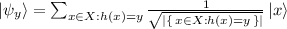. $\mathcal {A}$ could then use $\mathinner {|{\psi _y}\rangle }$ as a plaintext in the challenge phase, but note that $\mathcal {A}$ cannot reproduce $\mathinner {|{\psi _y}\rangle }$ for a given value y.

Both of the above examples are not reasonable in our scenario. Entanglement between $\mathcal {A}$ and $\mathcal {C}$ represents a sort of ‘quantum watermarking’ of messages, which goes beyond what a meaningful notion of indistinguishability should achieve. Knowledge of intermediate, unpredictable measurements also renders $\mathcal {A}$ too powerful, because it gives $\mathcal {A}$ access to information not available to $\mathcal {C}$ itself - e.g., in the example above $\mathcal {C}$ would not even know the value of y. As it is $\mathcal {C}$ who prepares the state to be encrypted, it is reasonable to assume that it is $\mathcal {C}$ who should know these intermediate measurements, not $\mathcal {A}$. In the example above, what $\mathcal {A}$ could see instead (provided he knows the circuit generating the state, as we assume in qIND) is that the plaintext is a mixture $\varPsi =\sum _y \psi _y$ for all possible values of y.

The possibility offered by gqIND of allowing the adversary to play the IND game with arbitrary states is certainly elegant from a theoretical point of view, but from the perspective of the quantum security of the kind of schemes we are considering, it is too broad in scope. The (c) model used in qIND, on the other hand, inherently provides guidelines and reasonable limitations on what a quantum adversary can or cannot do. Also, qIND is often easier to deal with: notice that in the (c) model, unlike in the (Q) model, $\mathcal {A}$ always receives back an unentangled state from a challenge query. In security reductions, this means that we can more easily simulate the challenger, and that we do not have to take care of measures of entanglement when analyzing the properties of quantum states - for example, indistinguishability of states can be shown by only resorting to the trace norm instead of the more general diamond norm.

Furthermore, it is important to notice that all our new results in Sect. 6 are unaffected by the choice of either qIND or gqIND. Our impossibility result from Theorem 6.3 holds for qIND, and hence also for gqIND because of Theorem 3.3. On the other hand, the security proof of Construction 6.6 (Theorem 6.9) is given for gqIND, and holds therefore also for qIND. In fact, it remains unclear whether a separation between qIND and gqIND can be found at all in the realm of classical encryption schemes. We leave this as an interesting open question.

Finally, we note that the q-IND-CPA-2 indistinguishability notion for secret-key encryption of quantum messages introduced by Broadbent and Jeffery [6, Appendix B] resembles our gqIND notion, and it is in fact equivalent to it in the case that the encryption operation is a symmetric-key classical functionality operating in type-(2) mode.

Theorem 3.4

(gqIND-qCPA $\Leftrightarrow$ q-IND-CPA-2). Let $\mathcal {E}$ be a symmetric-key encryption scheme. Then $\mathcal {E}$ is gqIND-qCPA secure if and only if $\mathcal {E}$ is q-IND-CPA-2 secure.

A proof of the above theorem can be found in the full version [9]. A generalization of q-IND-CPA-2 to arbitrary quantum encryption schemes, together with equivalent notions of quantum semantic security, was given and analyzed in [1]. All these security notions are given in the context of ‘fully quantum encryption’, in the sense that the encryption schemes considered in [6] and [1] are arbitrary quantum circuits acting natively on quantum data, while in this work we consider the quantum security of classical encryption schemes. The fully quantum homomorphic schemes which are shown to be secure in [6], and the other quantum encryption schemes shown to be secure in [1], do not fall into the category of classical encryption schemes which we are studying here. On the other hand, as Theorem 6.9 shows, our Construction 6.6 is the first known example of a classical symmetric-key encryption scheme which is secure even against these kinds of ‘fully quantum’ security notions.

4 New Notions of Quantum Semantic Security

In this section, we initiate the study of suitable definitions of semantic security in the quantum world. As in the classical case, we are particularly interested in notions that can be proven equivalent to some version of quantum indistinguishability. So these definitions actually describe the semantics of the equivalent IND notions. As in the classical case, we present these notions in the non-uniform model of computation.

Working towards a quantum SEM notion, we restrict our analysis to the SEM challenge phase. For the learning phase, we stick to the ‘qCPA learning phase’, as in Definition 2.5, where the adversary has access to a quantum encryption oracle. In the end, we give a definition for quantum semantic security under quantum chosen-plaintext attacks (qSEM-qCPA) which we later prove equivalent to qIND-qCPA, thereby adding semantics to our qIND-qCPA notion.

4.1 Classical Semantic Security Under Quantum CPA

As a first notion of semantic security in the quantum world, we consider what happens if, like in the IND-qCPA notion, we stick to the classical definition but we allow for a quantum chosen-plaintext-attack phase. The definition uses a SEM-qCPA game that is obtained by combining qCPA learning phases with a classical SEM challenge phase as defined in Sect. 2. As in the classical case, $\mathcal {A}$’s success probability is compared to that of a simulator $\mathcal {S}$ that plays in a reduced game: $\mathcal {S}$ gets no learning phase and during the challenge phase it only receives the advice $h_m(x)$, not the ciphertext.

Definition 4.1

(SEM-qCPA). A secret-key encryption scheme is called SEM-qCPA-secure if for every quantum polynomial-time machine $\mathcal {A}$, there exists a quantum polynomial-time machine $\mathcal {S}$ such that the challenge templates produced by $\mathcal {S}$ and $\mathcal {A}$ are identically distributed and the success probability of $\mathcal {A}$ winning the game defined by qCPA learning phases and a SEM challenge phase is negligibly close (in n) to the success probability of $\mathcal {S}$ winning the reduced game.

Spoiler. It is easy to see that the SEM-qCPA notion of semantic security is equivalent to IND-qCPA, see Theorem 5.1.

In the full version [9] we discuss what happens if one also allows quantum advice states in this scenario, and why this option would not add anything meaningful.

4.2 Quantum Semantic Security

We now define quantum semantic security under chosen-plaintext attacks (qSEM-qCPA). As in the classical case, we want the definition of semantic security to formally capture what we intuitively understand as a strong security notion. In the quantum case, there are several choices to be made. We start by giving our formal definition of quantum semantic security, and justify our choices afterwards.

Quantum SEM (qSEM) Challenge Phase: $\mathcal {A}$ sends to $\mathcal {C}$ a challenge template consisting of classical descriptions of

• a quantum circuit $G_m$ taking ${\text {poly}\,\left( n\right) }$-bit classical input and outputting m-qubit plaintext states,

• a quantum circuit $h_m$ taking m-qubit plaintexts as input and outputting ${\text {poly}\,\left( n\right) }$-qubit advice states,

• a quantum circuit $f_m$ taking m-qubit plaintexts as input and outputting ${\text {poly}\,\left( n\right) }$-qubit target states.

The challenger $\mathcal {C}$ samples $y \mathop {\longleftarrow }\limits ^{\$}\{0,1\}^{\text {poly}\,\left( n\right) }$ and computes two copies of the plaintext $\rho _y = G_m(y)$. One is used to compute auxiliary information $h_m(\rho _y)$ and one to compute the ciphertext $U_{\mathsf {Enc} _k} \, \rho _y \, U_{\mathsf {Enc} _k}^\dag$. $\mathcal {C}$ then replies with the pair $\left( U_{\mathsf {Enc} _k} \, \rho _y \, U_{\mathsf {Enc} _k}^\dag , h_m(\rho _y) \right)$. $\mathcal {A}$’s goal is to output $f_m(\rho _y)$. We say that $\mathcal {A}$ wins the qSEM-qCPA game if no quantum polynomial-time distinguisher can distinguish $\mathcal {A}$’s output from the target state $f_m(\rho _y)$ with non-negligible advantage.

In the reduced game, $\mathcal {S}$ receives no encryption, but only the auxiliary information $h_m(\rho _y)$ from $\mathcal {C}$. Analogously to the above case, $\mathcal {S}$ wins the qSEM-qCPA game if no quantum polynomial-time distinguisher can distinguish $\mathcal {S}$’s output from the target state $f_m(\rho _y)$ with non-negligible advantage.

Definition 4.2

(qSEM-qCPA). A secret-key encryption scheme is called qSEM-qCPA-secure if for every quantum polynomial-time machine $\mathcal {A}$, there exists a quantum polynomial-time machine $\mathcal {S}$ such that the challenge templates produced by $\mathcal {S}$ and $\mathcal {A}$ are identically distributed and the success probability of $\mathcal {A}$ winning the game defined by qCPA learning phases and a qSEM challenge phase is negligibly close (in n) to the success probability of $\mathcal {S}$ winning the reduced game.

When defining quantum semantic security, we have to deal with several issues: First, we have to define how the plaintext distribution is described. In the classical definition, the distribution is produced by a (classical) circuit $G_m$ running on uniform input bits. We take the same approach here, but let $G_m$ output m-qubit plaintexts.

The second question is how to define the advice function. While the input should be the plaintext quantum state $\rho _y$, the output could be either quantum or classical. We decided to allow quantum advice as it leads to a more general model and it includes classical outputs as a special case. In order for the challenger to compute both the encryption of the plaintext state $\rho _y$ and the advice state $h_m(\rho _y)$ without violation of the no-cloning theorem, we exploit how we generate the message state. We simply run $S_m$ twice on the same classical randomness y to generate two copies of the plaintext state $\rho _y$. Another option would have been to allow for entanglement between the plaintext message $\rho _y$ and the advice state $h_m(\rho _y)$. Allowing such entanglement would model side-channel information the attacker could obtain, for instance by learning the content of some internal register of the attacked device. However, the resulting notion would not be equivalent with qIND-qCPA anymore, because in qIND-qCPA, the challenge plaintexts are provided by their classical descriptions and can therefore not be entangled with the attacker.

Third, we have chosen to model the target function $f_m$ in the same way as the advice function $h_m$, i.e. we allow arbitrary quantum circuits that might output quantum states. The reasoning behind allowing quantum output is again to use the strongest possible, most general model. Allowing quantum output however leads to the problem that, in general, we cannot physically test anymore if an adversary $\mathcal {A}$ outputs exactly the result of the target function $f_m(\rho _y)$. One option would be to require $\mathcal {A}$’s output to be close to $f_m(\rho _y)$ in terms of their trace distance. But two quantum states can be quantum-polynomial-time indistinguishable even if their trace distance is large⁵. Since we are only interested in computational security notions, we solve this problem by requiring QPT indistinguishability as success condition for winning the SEM game.

Spoiler. Our qSEM-qCPA notion of semantic security is equivalent to qIND-qCPA, and unachievable for those schemes which leave the size of the message unchanged (like most block ciphers), see Sect. 6.1.

5 Relations

In this section we show relations between our new notions of indistinguishability and semantic security in the quantum world. It is already known [10, 11] that classically, IND-CPA and semantic security are equivalent. Our goal is to show a similar equivalence for our new notions, plus to show a hierarchy of equivalent security notions. Our results are summarized in Fig. 2.

Fig. 2.

The relations between notions of indistinguishability and semantic security in the quantum world (previously known results in gray).

Theorem 5.1

(IND-qCPA $\Leftrightarrow$ SEM-qCPA). Let $\mathcal {E}$ be a symmetric-key encryption scheme. Then $\mathcal {E}$ is IND-qCPA secure if and only if $\mathcal {E}$ is SEM-qCPA secure.

We split the proof of Theorem 5.1 into two propositions – one per direction. They closely follow the proofs for the classical case (see [10, Proof of Th. 5.4.11]), we recall them as they work as guidelines for the following proofs.

Proposition 5.2

(IND-qCPA $\Rightarrow$ SEM-qCPA).

Proposition 5.3

(SEM-qCPA $\Rightarrow$ IND-qCPA).

Proof

(of Proposition 5.2 – Sketch). The idea of the proof is to hand $\mathcal {A}$’s circuit as non-uniform advice to the simulator $\mathcal {S}$. $\mathcal {S}$ runs $\mathcal {A}$’s circuit and impersonates the challenger $\mathcal {C}$ by generating a new key and answering all of $\mathcal {A}$’s queries using this key. When it comes to the challenge query, $\mathcal {S}$ encrypts the $1\ldots 1$ string of the same length as the original message. It follows from the indistinguishability of encryptions that the adversary’s success probability in this game must be negligibly close to its success probability in the real semantic-security game, which concludes the proof. The only difference in the -qCPA case is that $\mathcal {A}$ and $\mathcal {S}$ are quantum circuits, and that $\mathcal {S}$ has to emulate the quantum encryption oracle instead of a classical one.   $\square$

Proof

(of Proposition 5.3 ). We recall here the full proof as it is short. Assume there exists an efficient distinguisher $\mathcal {A}$ against the IND-qCPA security of $\mathcal {E}$. Then we show how to construct an oracle machine $\mathcal {M} ^\mathcal {A}$ that has access to $\mathcal {A}$ and breaks the SEM-qCPA security of the scheme. $\mathcal {M} ^\mathcal {A}$ runs $\mathcal {A}$, emulating the quantum encryption oracle by simply forwarding all the qCPA queries to its own oracle. As $\mathcal {A}$ executes an IND challenge query on m-bit messages $(x_0,x_1), \mathcal {M} ^\mathcal {A}$ produces the SEM template $(G_m,h_m,f_m)$ with $G_m$ describing the uniform distribution over (or any other function such that $h_m(x_0)=h_m(x_1)$), and $f_m$ a function that fulfills $f_m(x_0)=0$ and $f_m(x_1)=1$ (i.e., the distinguishing function). Then $\mathcal {M} ^\mathcal {A}$ performs a SEM challenge query with this template, and given challenge ciphertext c, uses it to answer $\mathcal {A}$’s query. If, at that point, $\mathcal {A}$ performs more qCPA queries, $\mathcal {M} ^\mathcal {A}$ answers again by forwarding all these queries to its own oracle. Finally, $\mathcal {M} ^\mathcal {A}$ outputs $\mathcal {A}$’s output. As $\mathcal {A}$ distinguishes encryptions of $x_0$ and $x_1$ with non-negligible success probability, $\mathcal {A}$ will return the correct value of $f_m$ with recognizably higher probability than guessing. As $h_m$ is independent of the encrypted message, no simulator can do better than guessing. Hence, $\mathcal {M} ^\mathcal {A}$ has a non-negligible advantage to output the right value of $f_m$.    $\square$

Theorem 5.4

(qIND-qCPA $\Leftrightarrow$ qSEM-qCPA). Let $\mathcal {E}$ be a symmetric-key encryption scheme. Then $\mathcal {E}$ is qIND-qCPA secure if and only if $\mathcal {E}$ is qSEM-qCPA secure.

Again, we split the proof of Theorem 5.4 into two propositions.

Proposition 5.5

(qIND-qCPA $\Rightarrow$ qSEM-qCPA).

Proposition 5.6

(qSEM-qCPA $\Rightarrow$ qIND-qCPA).

Proof

(of Proposition 5.5 – Sketch). The proof follows that of Proposition 5.2, with some careful observations. Since $\mathcal {A}$ is a QPT adversary against the qSEM-qCPA game, $\mathcal {A}$’s circuit has a short classical representation $\xi$. So $\mathcal {S}$ gets $\xi$ as non-uniform advice and hence can implement and run $\mathcal {A}$. The simulator $\mathcal {S}$ simulates $\mathcal {C}$ for $\mathcal {A}$ by generating a new key and answering all of $\mathcal {A}$’s qCPA queries. When it comes to the challenge query, $\mathcal {A}$ produces a qSEM template, which $\mathcal {S}$ forwards to the real $\mathcal {C}$. Then $\mathcal {S}$ forwards $\mathcal {C}$’s reply, plus a bogus encrypted state (e.g., $U_{\mathsf {Enc} _k} \, \mathinner {|{1\ldots 1}\rangle }$), to $\mathcal {A}$. If at this point $\mathcal {A}$ outputs a state $\varphi$ which can be efficiently distinguished from the correct $f_m(\rho _y)$ computed by the real $\mathcal {C}$, we would have an efficient distinguisher against the qIND-qCPA security of the scheme. Hence, $\mathcal {A}$’s (and therefore also $\mathcal {S}$’s) output must be indistinguishable from $f_m(\rho _y)$ for any QPT distinguisher, which concludes the proof.   $\square$

Proof

(of Proposition 5.6 ). This is also similar to the proof of Proposition 5.3. Given an efficient distinguisher $\mathcal {A}$ for the qIND-qCPA game, our adversary for the qSEM-qCPA game is an oracle machine $\mathcal {M} ^\mathcal {A}$ running $\mathcal {A}$ and acting as follows. Concerning $\mathcal {A}$’s qCPA queries, as usual $\mathcal {M} ^\mathcal {A}$ just forwards everything to the qSEM-qCPA challenger $\mathcal {C}$. When $\mathcal {A}$ performs a challenge qIND query by sending the classical descriptions of two states $\varphi _0$ and $\varphi _1$, $\mathcal {M} ^\mathcal {A}$ prepares the qSEM template $(G_m,h_m,f_m)$, with $G_m$ outputing $\varphi _0$ for half of the possible y values and $\varphi _1$ for the other half, $h_m(\rho _y)=1^n$, and $f_m$ the identity map $f_m(\rho _y)=\rho _y$. Then $\mathcal {M} ^\mathcal {A}$ performs a qSEM challenge query with this template. Given challenge ciphertext state $U_{\mathsf {Enc} _k} \, \varphi _b \, U_{\mathsf {Enc} _k}^\dag$ (for $b\in \{0,1\}$), he forwards it as an answer to $\mathcal {A}$’s challenge query. As $\mathcal {A}$ distinguishes $U_{\mathsf {Enc} _k} \, \varphi _0 \, U_{\mathsf {Enc} _k}^\dag$ from $U_{\mathsf {Enc} _k} \, \varphi _1\, U_{\mathsf {Enc} _k}^\dag$ with non-negligible success probability, $\mathcal {A}$ returns the correct value of b with non-negligible advantage over guessing. Then $\mathcal {M} ^\mathcal {A}$, having recorded a copy of the classical descriptions of $\varphi _0$ and $\varphi _1$, is able to compute the state $f_m(\varphi _b)$ exactly, and consequently win the qSEM-qCPA game with non-negligible advantage. As $h_m$ generates the same advice state $h_m(\rho _y)=1^n$ independently of the encrypted message, no simulator can do better than guessing the plaintext. This concludes the proof.   $\square$

Finally, we show the separation result between the two classes of security we have identified (we show it between IND-qCPA and qIND-qCPA). This shows that qIND-qCPA (and equivalently qSEM-qCPA) is a strictly stronger notion than IND-qCPA (which is equivalent to SEM-qCPA).

Theorem 5.7

(IND-qCPA $\nRightarrow$ qIND-qCPA). There exists a symmetric-key encryption scheme $\mathcal {E}$ which is IND-qCPA secure but not qIND-qCPA secure.

Proof

(of Theorem 5.7 ). The scheme we use as a counterexample is the one from [10] (Construction 5.3.9). It has been proven in [4] that this scheme is IND-qCPA secure if the used PRF is post-quantum secure. We exhibit a distinguisher $\mathcal {A}$ which breaks the qIND-qCPA security of this scheme with high probability. For ease of notation we restrict to the case of single-bit messages 0 and 1. $\mathcal {A}$ will simply choose as challenge states: $\mathinner {|{\varphi _0}\rangle } = H\mathinner {|{0}\rangle } = \frac{1}{\sqrt{2}}\mathinner {|{0}\rangle } + \frac{1}{\sqrt{2}}\mathinner {|{1}\rangle }$, and $\mathinner {|{\varphi _1}\rangle } = H\mathinner {|{1}\rangle } = \frac{1}{\sqrt{2}}\mathinner {|{0}\rangle } - \frac{1}{\sqrt{2}}\mathinner {|{1}\rangle }$. When the challenger $\mathcal {C}$ applies the type-2 transformation to either of these two states, it is easy to see that in any case the state is left unchanged. This is because $U_{\mathsf {Enc} _k}$ just applies a permutation in the space of the basis elements, but $\mathinner {|{\varphi _0}\rangle }$ and $\mathinner {|{\varphi _1}\rangle }$ have the same amplitudes on all their components, except for the sign. As these two states are orthogonal, they can be reliably distinguished by the adversary $\mathcal {A}$ who can then win the qIND-qCPA game with probability 1.   $\square$

The above proof can be generalized to message states of arbitrary length, as our impossibility result in Sect. 6.1 shows.

6 Impossibility and Achievability Results

In this section we show that qIND-qCPA (and equivalently qSEM-qCPA) is impossible to achieve for encryption schemes which do not expand the message (such as stream ciphers and many block ciphers, without considering the randomness part in the ciphertext). Therefore, for a scheme to be secure according to this new definition, it is necessary (but not sufficient) to increase the message size during the encryption. Interestingly, such an increase happens in most public-key post-quantum encryption schemes, like for example LWE based schemes [18] or the McEliece scheme [19].

Then we propose a construction of a qIND-qCPA–secure symmetric-key encryption scheme. Our construction works for any (quantum-secure) pseudorandom permutation (PRP). Given that block ciphers are usually modelled as PRPs, it seems reasonable to assume that we can obtain a secure scheme when using block ciphers with sufficiently large key and block size. Hence, our construction can be used to patch existing schemes, or as a guideline in the design of quantum-secure encryption schemes from block ciphers.

6.1 Impossibility Result

First we formally define what it means for a cipher to expand or keep constant the message size by defining the core function of a (secret-key) encryption scheme. Intuitively, the definition splits the ciphertext into the randomness and a part carrying the message-dependent information. This definition covers most encryption schemes in the literature.

Definition 6.1

(Core Function). Let $(\mathsf {Gen},\mathsf {Enc},\mathsf {Dec})$ be a secret-key encryption scheme. We call the function $f:\mathcal {K}\times \{0,1\}^\tau \times \mathcal {M}\rightarrow \mathcal {Y}$ the core function of the encryption scheme if, for some $\tau \in \mathbb {N}$:

• for all $k\in \mathcal {K}$ and $x \in \mathcal {M}$, $\mathsf {Enc} _k(x)$ can be written as (r, f(k, r, x)), where $r\in \{0,1\}^\tau$ is independent of the message; and

• there exists a function $f'$ such that for all $k\in \mathcal {K}, r\in \{0,1\}^\tau , x\in \mathcal {M}$, we have: $f'(k,r,f(k,x,r)) = x$.

For example, in case of Construction 5.3.9 from [10] (where $Enc_k(x)$ is defined as $(r,F_k(r)\oplus x)$ for a PRF $F$) the core function is $f(k,r,x) = F_{k}(r) \oplus x$, with $f'(k,r,z) = z \oplus F_k(r)$.

Definition 6.2

(Quasi–Length-Preserving Encryption). We call a secret-key encryption scheme with core function f quasi–length-preserving if

$$\begin{aligned} \forall x \in \mathcal {M}, r \in \{0,1\}^\tau , k \in \mathcal {K}\Rightarrow |f(k,x,r)| = |x|, \end{aligned}$$

i.e., if the output of the core function has the same bit length as the message.

Continuing the above example, Construction 5.3.9 from [10] is quasi–length-preserving.

The crucial observation is the following: For a quasi–length-preserving encryption scheme, the space of possible input and (core function) output bitstrings (with respect to plaintext and ciphertext) coincide, therefore these ciphers act as permutations on this space. This means that if we start with an input state which is a superposition of all the possible basis states, all of them with the same amplitude, this state will be unchanged by the unitary type-2 encryption operation (because it will just ‘shuffle’ in the basis-state space amplitudes which are exactly the same).

Theorem 6.3

(Impossibility Result). No quasi–length-preserving secret-key encryption scheme can be qIND secure.

Proof

Let $(\mathsf {Gen},\mathsf {Enc},\mathsf {Dec})$ be a quasi–length-preserving scheme. We show an attack that is a generalization of the distinguishing attack in Theorem 5.7.

• 1. for m-bit message strings, the distinguisher $\mathcal {D}$ sets the two plaintext states for the qIND- game to be: $\mathinner {|{\varphi _0}\rangle } = H \mathinner {|{0^m}\rangle }, \mathinner {|{\varphi _1}\rangle } = H \mathinner {|{1^m}\rangle }$, where H is the m-fold tensor Hadamard transformation. Notice that both these states admit efficient classical representations, and are thus allowed in the qIND game.

• 2. The challenger flips a random bit b and returns $\mathinner {|{\psi }\rangle } = U_{\mathsf {Enc} _k}\mathinner {|{\varphi _b}\rangle }$.

• 3. $\mathcal {D}$ applies H to the core-function part of the ciphertext $\mathinner {|{\psi }\rangle }$ and measures it in the computational basis. $\mathcal {D}$ outputs 0 if and only if the outcome is $0^m$, and outputs 1 otherwise.

As already observed, applying $U_{\mathsf {Enc} _k}$ to $H \mathinner {|{0^m}\rangle }$ leaves the state untouched: since the encryption oracle merely performs a permutation in the basis space, and since $\mathinner {|{\varphi _0}\rangle }$ is a superposition of every basis element with the same amplitude, it follows that whenever b is equal to 0, the ciphertext state will be unchanged. In this case, after applying the self-inverse transformation H again, $\mathcal {D}$ obtains measurement outcome $0^m$ with probability 1. On the other hand, if $b=1$, $\mathinner {|{\varphi _1}\rangle } = \frac{1}{2^{m/2}}\sum _y (-1)^{y \cdot 1^m} \mathinner {|{y}\rangle }$ where $a \cdot b$ denotes the bitwise inner product between a and b. Hence, $\mathinner {|{\varphi _1}\rangle }$ is a superposition of every basis element where (depending on the parity of y) half of the elements have a positive amplitude and the other half have a negative one, but all of them will be equal in absolute value. Applying $U_{\mathsf {Enc},k}$ to this state, results in $\frac{1}{2^{m/2}}\sum _y (-1)^{y \cdot 1^m} \mathinner {|{\mathsf {Enc} _k(y)}\rangle }$. After re-applying H, the amplitude of the basis state $\mathinner {|{0^m}\rangle }$ becomes $\sum _y (-1)^{y \cdot 1^m + \mathsf {Enc} _k(y) \cdot 0^m}$ which is easily calculated to be 0. Hence, the above attack gives $\mathcal {D}$ a way of perfectly distinguishing between encryptions of the two plaintext states.    $\square$

Notice that the above attack also works if $\mathcal {A}$ is allowed to send quantum states to $\mathcal {C}$ directly. Therefore, it also holds for the gqIND notion of quantum indistinguishability described in Sect. 3. In particular, the above theorem shows that [10, Construction 5.3.9], which in [4] was shown to be IND-qCPA if the used PRF is quantum secure, does not fulfill qIND, nor gqIND.

This attack is a consequence of the well-known fact that, in order to perfectly (information-theoretically) encrypt a single quantum bit, two bits of classical information are needed: one to hide the basis bit, and one to hide the phase (i.e. the signs of the amplitudes). The fact that we are restricted to quantum operations of the form $U_{\mathsf {Enc} _k}$ - that is, quantum instantiations of classical encryptions - means that we cannot afford to hide the phase as well, and this restriction allows for an easy distinguishing procedure.

6.2 Secure Construction

Here we propose a construction of a qIND-qCPA secure symmetric-key encryption scheme from any family of quantum-secure pseudorandom permutations (see the full version [9] for formal definitions).

Construction 6.4

For security parameter n, let $m= {\text {poly}\,\left( n\right) }$ and $\tau = {\text {poly}\,\left( n\right) }$. Consider an efficient family of permutations $\varPi _{m+\tau } = (\mathcal {I}, \varPi , \varPi ^{-1})$ with key space $\mathcal {K}_\varPi$ that operates on bit strings of length $m+\tau$, and consider a plaintext message space $\mathcal {M}= \{0,1\}^m$, key space $\mathcal {K}= \mathcal {K}_\varPi$, and ciphertext space $\mathcal {C} =\{0,1\}^{m+\tau }$. The construction is given by the following algorithms:

• Key generation algorithm $k \longleftarrow \mathsf {Gen} (1^n)$ : on input of security parameter n, the key generation algorithm runs $k\longleftarrow \mathcal {I} (1^{m+\tau })$ and returns secret key k.

• Encryption algorithm $y \longleftarrow \mathsf {Enc} _k(x)$ : on input of message $x \in \mathcal {M}$ and key $k \in \mathcal {K}$, the encryption algorithm samples a $\tau$-bit string $r\mathop {\longleftarrow }\limits ^{\$}\{0,1\}^\tau$ uniformly at random, and outputs $y = \pi _k(x\Vert r)$ ($\Vert$ denotes string concatenation).

• Decryption algorithm $x \longleftarrow \mathsf {Dec} _k(y)$ : on input of ciphertext $y \in \mathcal {C}$ and key $k \in \mathcal {K}$, the decryption algorithm first runs $x' = \pi ^{-1}_k(y)$, and then returns the first m bits of $x'$.

The soundness of the construction can be easily checked. The security is stated in the following theorem.

Theorem 6.5

(qIND-qCPA Security of Construction 6.4 ). If $\varPi _{m+\tau }$ is a family of quantum-secure pseudorandom permutations (qPRP), then the encryption scheme $(\mathsf {Gen},\mathsf {Enc},\mathsf {Dec})$ defined in Construction 6.4 is qIND-qCPA secure.

In the next section, we prove the security of a more powerful scheme which includes the above theorem as special case of a single message block.

6.3 Length Extension

Construction 6.4 has the drawback that the message length is upper bounded by the input length of the qPRP (minus the bit length of the randomness). However, like in the case of block ciphers, we can overcome this issue with a mode of operation. More specifically, we can handle arbitrary message lengths by splitting the message into m-bit blocks and applying the encryption algorithm of Construction 6.4 independently to each message block (using the same key but new randomness for each block). This procedure is akin to a ‘randomized ECB mode’, in the sense that each message block is processed separately, like in the ECB (Electronic Code Book) mode, but in our case the underlying cipher is inherently randomized (since we use fresh randomness for each block), so we can still achieve qCPA security. For simplicity we consider only message lengths which are multiples of m. The construction can be generalized to arbitrary message lengths using standard padding techniques. Moreover, the randomness for every block can be generated efficiently using a random seed and a post-quantum secure PRNG.

Construction 6.6

For security parameter n, let $m= {\text {poly}\,\left( n\right) }$ and $\tau = {\text {poly}\,\left( n\right) }$. Consider an efficient family of permutations $\varPi _{m+\tau } = (\mathcal {I}, \varPi , \varPi ^{-1})$ with key space $\mathcal {K}_\varPi$ that operates on bit strings of length $m+\tau$, and consider a plaintext message space $\mathcal {M}= \{0,1\}^{\mu m}$ for $\mu \in \mathbb {N}, \mu = {\text {poly}\,\left( n\right) }$, key space $\mathcal {K}= \mathcal {K}_\varPi$, and ciphertext space $\mathcal {C} =\{0,1\}^{\mu (m+\tau )}$. The construction is given by the following algorithms:

• Key generation algorithm $k \longleftarrow \mathsf {Gen} (1^n)$ : on input of security parameter n, the key generation algorithm runs $k\longleftarrow \mathcal {I} (1^{m+\tau })$ and returns secret key k.

• Encryption algorithm $y \longleftarrow \mathsf {Enc} _k(x)$ : on input of message $x \in \mathcal {M}$ and key $k \in \mathcal {K}$, the encryption algorithm splits x into $\mu$ m-bit blocks $x_1, \ldots , x_\mu$. For each block $x_i$, the encryption algorithm samples a new $\tau$-bit string $r_i\mathop {\longleftarrow }\limits ^{\$}\{0,1\}^\tau$ uniformly at random, and outputs $y_i = \pi _k(x_i\Vert r_i)$ ($\Vert$ denotes string concatenation). The ciphertext is $y = y_1 \Vert \ldots \Vert y_\mu$.

• Decryption algorithm $x \longleftarrow \mathsf {Dec} _k(y)$ : on input of ciphertext $y \in \mathcal {C}$ and key $k \in \mathcal {K}$, the decryption algorithm first splits y into $\mu$ $m+\tau$-bit blocks $y_1, \ldots , y_\mu$. Then, it runs $x'_i = (\pi ^{-1}_k(y_i))_m$ for each block (where $(s)_m$ refers to taking the first m bits of bit string s). It returns the plaintext $x' = x'_1, \ldots , x'_\mu$.

The soundness of the construction can be checked easily. For the security, we observe that splitting a $\mu m$-qubit plaintext state into $\mu$ blocks of m-qubits can introduce entanglement between the blocks. We will address this issue through the following technical lemma.

Lemma 6.7

Let $\mathcal {E}$ be the quantum channel that takes as input an arbitrary m-qubit state, attaches another $\tau$ qubits in state $\mathinner {|{0}\rangle }$, and then applies a permutation picked uniformly at random from $S_{2^{m+\tau }}$ to the computational basis space. Let $\mathcal {T}$ be the constant channel which maps any m-qubit state to the totally mixed state on $m+\tau$ qubits. Then, $\Vert \mathcal {E} - \mathcal {T} \Vert _{\diamond } \le 2^{-\tau +2}$.

Proof

In order to consider the fact that the m-qubit input state might be entangled with something else, we have to start with a purification of such a state. Formally, this is a bipartite pure 2m-qubit state $\mathinner {|{\phi }\rangle }_{XY} = \sum _{x,y} \alpha _{x,y} \mathinner {|{x}\rangle }_X \mathinner {|{y}\rangle }_Y$ whose m-qubit Y register is input into the channel and gets transformed into $id_X \otimes \mathcal {E}({|\phi \rangle \!\langle \phi |}) = {{\mathrm{tr}}}_{\varPi } {|\psi \rangle \!\langle \psi |}$ where

$$\begin{aligned} \mathinner {|{\psi }\rangle } = \sum _{x \in \{0,1\}^m,y \in \{0,1\}^m,\pi \in S_{2^{m+\tau }}} \alpha _{x,y} \mathinner {|{x}\rangle }_X \mathinner {|{\pi (y || 0)}\rangle }_C \mathinner {|{\pi }\rangle }_{\varPi }. \end{aligned}$$

By definition of the diamond-norm, we have to show that for any 2m-qubit state $\rho$, we have that $\Vert (id \otimes \mathcal {E})(\rho ) - (id \otimes \mathcal {T})(\rho )\Vert _{{{\mathrm{tr}}}} \le 2^{-\tau +2}$. Due to the convexity of the trace distance, we may assume that $\rho = {|\phi \rangle \!\langle \phi |}$ is pure with $\mathinner {|{\phi }\rangle }_{XY} = \sum _{x,y} \alpha _{x,y} \mathinner {|{x}\rangle }_X \mathinner {|{y}\rangle }_Y$. Hence, we obtain

$$\begin{aligned} (id_X \otimes \mathcal {E})({|\phi \rangle \!\langle \phi |})&= {{\mathrm{tr}}}_{\varPi } {|\psi \rangle \!\langle \psi |} \\&=\frac{1}{2^{m+\tau }!} \sum _{x,x',y,y',\pi } \alpha _{x,y} \overline{\alpha _{x',y'}} {|x\rangle \!\langle x'|}_X \otimes \mathinner {|{\pi (y \Vert 0)}\rangle }\mathinner {\langle { \pi (y' \Vert 0)}|}_C\\&=\frac{1}{2^{m+\tau }!} \sum _{x,x',y} \alpha _{x,y} \overline{\alpha _{x',y}} {|x\rangle \!\langle x'|}_X \otimes \sum _\pi \mathinner {|{\pi (y \Vert 0)}\rangle }\mathinner {\langle { \pi (y \Vert 0)}|}_C\\&\quad + \frac{1}{2^{m+\tau }!} \sum _{x,x',y \ne y'} \alpha _{x,y} \overline{\alpha _{x',y'}} {|x\rangle \!\langle x'|}_X \otimes \sum _\pi \mathinner {|{\pi (y \Vert 0)}\rangle }\mathinner {\langle { \pi (y' \Vert 0)}|}_C \\&=\sum _{x,x',y} \alpha _{x,y} \overline{\alpha _{x',y}} {|x\rangle \!\langle x'|}_X \otimes \frac{1}{2^{m+\tau }} \sum _z {|z\rangle \!\langle z|}_C\\&\quad + \sum _{x,x',y \ne y'} \alpha _{x,y} \overline{\alpha _{x',y'}} {|x\rangle \!\langle x'|}_X \otimes \frac{1}{2^{m+\tau }(2^{m+\tau }-1)}\sum _{z \ne z'} {|z\rangle \!\langle z'|}_C\\&={{\mathrm{tr}}}_Y {|\phi \rangle \!\langle \phi |} \otimes \tau _C + \chi _{XC}\\&=(id_X \otimes \mathcal {T}) ({|\phi \rangle \!\langle \phi |}) + \chi _{XC}, \end{aligned}$$

where we defined the “difference state”

$$\begin{aligned} \chi _{XC} := \sum _{x,x',y \ne y'} \alpha _{x,y} \overline{\alpha _{x',y'}} {|x\rangle \!\langle x'|}_X \otimes \frac{1}{2^{m+\tau }(2^{m+\tau }-1)}\sum _{z \ne z'} {|z\rangle \!\langle z'|}_C. \end{aligned}$$

In order to conclude, it remains to show that $\Vert \chi _{XC} \Vert _{{{\mathrm{tr}}}} \le 2^{-\tau +2}$. For the C-register $\chi _C = \frac{1}{2^{m+\tau }(2^{m+\tau }-1)}\sum _{z \ne z'} {|z\rangle \!\langle z'|}_C$, one can verify that the $2^{m+\tau }$ eigenvalues are $(c \cdot (2^{m+\tau }-1),-c,-c,\ldots ,-c)$ where $c:=\frac{1}{2^{m+\tau }(2^{m+\tau }-1)}$. Hence, the trace norm (which is the sum of the absolute eigenvalues) is exactly $c \cdot 2(2^{m+\tau }-1) = 2^{-m-\tau +1}$.

For the X-register, we split $\chi _X$ into two parts $\chi _X = \xi _X - \xi '_X$ where

$$\begin{aligned} \xi _X&:= \sum _{x,x'} {|x\rangle \!\langle x'|} \sum _{y,y'} \alpha _{x,y} \overline{\alpha _{x',y'}},\\ \xi '_X&:= \sum _{x,x'} {|x\rangle \!\langle x'|} \sum _{y} \alpha _{x,y} \overline{\alpha _{x',y}}, \end{aligned}$$

and use the triangle inequality for the trace norm $\Vert \chi _X\Vert _{{{\mathrm{tr}}}} = \Vert \xi _X - \xi '_X\Vert _{{{\mathrm{tr}}}} \le \Vert \xi _X\Vert _{{{\mathrm{tr}}}} + \Vert \xi '_{X}\Vert _{{{\mathrm{tr}}}}$. Observe that $\Vert \xi _X \Vert _{{{\mathrm{tr}}}} = \Vert \sum _{x,y} \alpha _{x,y} \mathinner {|{x}\rangle } \sum _{x',y'} \overline{\alpha _{x',y'}} \mathinner {\langle {x'}|} \Vert _{{{\mathrm{tr}}}} = \Vert {|s\rangle \!\langle s|} \Vert _{{{\mathrm{tr}}}}$ for the (non-normalized) vector $\mathinner {|{s}\rangle } := \sum _{x,y} \alpha _{x,y} \mathinner {|{x}\rangle }$. Hence, the trace-norm $\Vert \xi _X \Vert _{{{\mathrm{tr}}}} = | \mathinner {\langle {s\mid s}\rangle } | = \sum _x | \sum _y \alpha _{x,y} |^2 \le \sum _x \sum _y |\alpha _{x,y}|^2 \cdot 2^m = 2^m$ by the Cauchy-Schwarz inequality and the normalization of the $\alpha _{x,y}$’s. Furthermore, we note that $\xi '_X$ is exactly the reduced density matrix of $\mathinner {|{\phi }\rangle }_{XY}$ after tracing out the Y register. Hence, $\xi '_X$ is positive semi-definite and its trace norm is equal to its trace which is 1. In summary, we have shown that

$$\begin{aligned} \Vert \chi _{XC} \Vert _{{{\mathrm{tr}}}}&= \Vert \chi _X \Vert _{{{\mathrm{tr}}}} \cdot \Vert \chi _C \Vert _{{{\mathrm{tr}}}} \le (\Vert \xi _X - \xi '_X \Vert _{{{\mathrm{tr}}}}) \cdot 2^{-m-\tau +1}\\&\le (\Vert \xi _X\Vert _{{{\mathrm{tr}}}} + \Vert \xi '_X \Vert _{{{\mathrm{tr}}}}) \cdot 2^{-m-\tau +1} \le (2^m + 1) \cdot 2^{-m-\tau +1} \le 2^{-\tau +2}. \end{aligned}$$

   $\square$

If we consider a slightly different encryption channel $\mathcal {E}^T$ which still maps m qubits to $m+\tau$ qubits but where the permutation $\pi$ is not picked uniformly from $S_{2^{m+\tau }}$, but instead we are guaranteed that a certain set $T \subset \{0,1\}^{m+\tau }$ of outputs never occurs, we can consider such permutations w.l.o.g. as picked uniformly at random from a smaller set $S_{2^{m+\tau }-|T|}$. In this setting, we are interested in the distance of the encryption operation $\mathcal {E}^T$ from the slightly different constant channel $\mathcal {T}^T$ which maps all inputs to the $(m+\tau )$-qubit state which is completely mixed on the smaller set $\{0,1\}^{m+\tau } \setminus T$. By modifying slightly the proof of Lemma 6.7 we get the following.

Corollary 6.8

Let $\mathcal {E}^T$ and $\mathcal {T}^T$ be the channels defined above. Then,

$$\begin{aligned} \Vert \mathcal {E}^T - \mathcal {T}^T \Vert _{\diamond } \le \frac{4}{2^{\tau } - |T|/2^m}. \end{aligned}$$

(3)

We can now prove the security of Construction 6.6. We give the proof for gqIND-qCPA, and then qIND-qCPA follows immediately from Theorem 3.3.

Theorem 6.9

(gqIND-qCPA Security of Construction 6.6 ). If $\varPi _{m+\tau }$ is a family of quantum-secure pseudorandom permutations (qPRP), then the encryption scheme $(\mathsf {Gen},\mathsf {Enc},\mathsf {Dec})$ defined in Construction 6.6 is gqIND-qCPA secure.

Proof

We want to show that no QPT distinguisher $\mathcal {D}$ can win the gqIND-qCPA game with probability substantially better than guessing. We first transform the game through a short game-hopping sequence into an indistinguishable game for which we can bound the success probability of any such $\mathcal {D}$.

Game 0. This is the original gqIND-qCPA game.

Game 1. This is like Game 0, but instead of using a permutation drawn from the qPRP family $\varPi _{m+\tau }$, a random permutation $\pi \in S_{2^{m+\tau }}$ is chosen from the set of all permutations over $\{0,1\}^{m+\tau }$. The difference in the success probability of $\mathcal {D}$ winning one or the other of these two games is negligible. Otherwise, we could use $\mathcal {D}$ to distinguish a random permutation drawn from $\varPi _{m+\tau }$ from one drawn from $S_{2^{m+\tau }}$. This would contradict the assumption that $\varPi _{m+\tau }$ is a qPRP.

Game 2. This is like Game 1, but $\mathcal {D}$ is guaranteed that the randomness used for each encryption query are $\mu$ new random $\tau$-bit strings that were not used before. In other words, the challenger keeps track of all random values used so far and excludes those when sampling a new randomness. Since in Game 1 the same randomness is sampled twice only with negligible probability, the probability of winning these two games differs by at most a negligible amount.

Game 3. This is like Game 2 except that the answer to each query asked by $\mathcal {D}$ also contains the randomness $r_1,\ldots ,r_{\mu }$ used by the challenger for answering that query. Clearly, $\mathcal {D}$ ’s probability of winning this game is at least the probability of winning Game 2.

When the modified gqIND game 3 starts, $\mathcal {D}$ chooses two different plaintext states and sends them to the challenger, who will then choose one of them and send it back encrypted with fresh randomness $\hat{r}_1, \ldots ,\hat{r}_{\mu }$. Let Q denote the set of $q \cdot \mu = poly(n)$ query values used during the previous qCPA-phase. We have to consider that from this phase, $\mathcal {D}$ knows a set $T \subset \{0,1\}^{m+\tau }$ of ‘taken’ outputs, i.e. he knows that any $\pi (x\Vert \hat{r}_i)$ will not take one of these values as $\hat{r}_i$ has not been used before. So, from the adversary’s point of view, $\pi$ is a permutation randomly chosen from $S'$, the set of those permutations over $\{0,1\}^{m+\tau }$ that fix these |T| values. In order to simplify the proof, we will consider a very conservative bound where $|T| = q \cdot \mu \cdot 2^m$, and the size of $S'$ is $|S'| = (2^{m+\tau }-|T|)!$ (notice that this bound is very conservative because it assumes that the adversary learns $2^m$ different (classical) ciphertexts for every of the $q \cdot \mu$ ‘taken’ randomnesses, but as we will see, this knowledge will be still insufficient to win the game).

By construction, the encryption of a $\mu m$-qubit (possibly mixed) state $\sigma$ is performed in $\mu$ separate blocks of m qubits each. We are guaranteed that fresh randomness is used in each block, hence it follows from Corollary 6.8 that $\mathsf {Enc} _k(\sigma )$ is negligibly close to the ciphertext state where the first $m+\tau$ qubits are replaced with the completely mixed state (by noting that $|T|/2^m = q \cdot \mu$ is polynomial in n in our case, and hence the right-hand side of (3) is negligible). Another application of Corollary 6.8 gives negligible closeness to the ciphertext state where the first $2(m+\tau )$ qubits are replaced with the completely mixed state etc. After $\mu$ applications of Corollary 6.8, we have shown that $\mathsf {Enc} _k(\sigma )$ is negligibly close to the totally mixed state on $\mu (m+\tau )$ qubits. As this argument can be made for any cleartext state $\sigma$, we have shown that from $\mathcal {D}$’s point of view, all encrypted states are negligibly close to the totally mixed state and therefore cannot be distinguished.    $\square$

Corollary 6.10

(qIND-qCPA Security of Construction 6.6 ). If $\varPi _{m+\tau }$ is a family of quantum-secure pseudorandom permutations (qPRP), then the encryption scheme $(\mathsf {Gen},\mathsf {Enc},\mathsf {Dec})$ defined in Construction 6.6 is qIND-qCPA secure.

7 Conclusions and Further Directions

We believe that many of the current security notions used in different areas of cryptography are unsatisfying in case quantum computers become reality. In this respect, our work contributes to a better understanding of which properties are important for the long-term security of modern cryptographic primitives. Our work leads to many interesting follow-up questions.

There are many other directions to investigate, once the basic framework of ‘indistinguishability versus semantic security’ presented in this work is completed. A natural direction is to look at quantum CCA1 security in this framework. This topic was also initiated in [4] relative to the IND-qCPA model; it would be interesting to extend the definition of CCA1 security to stronger notions obtained by starting from our qIND-qCPA model.

In Sect. 3.3 we left open the interesting question on whether it is possible at all to find a separating example between the notions of qIND and gqIND. That is, find a symmetric-key encryption scheme $\mathcal {E}$ which is qIND-secure, but not gqIND-secure. Finding such an example (or provable lack of) would shed further light on the security model we consider.

We have so far not taken into account models where the adversary is allowed to initialize the ancilla qubits used in the encryption operation used by the challenger (i.e. the $\mathinner {|{y}\rangle }$ in $\mathinner {|{x,y}\rangle } \mapsto \mathinner {|{x,y \oplus \mathsf {Enc} _k(x)}\rangle }$). These models lead to the study of quantum fault attacks, because they model cases where the adversary is able to ‘watermark’ or tamper with part of the challenger’s internal memory. Moreover, we have not considered superpositions of keys or randomness: these lead to a quantum study of weak-key and bad-randomness models. The authors of this paper are not aware of any results in these directions.

One outstanding open problem is to define CCA2 (adaptive chosen ciphertext attack) security in the quantum world. The problem is that in the CCA2 game the challenger has to ensure that the attacker does not ask for a decryption of the actual challenge ciphertext leading to a trivial break. While this is easily implemented in the classical world, it raises several issues in the quantum world. What does it mean for a ciphertext to be different from the challenge ciphertext? And, more importantly: How can the challenger check? There might be several reasonable ways to solve the first issue but, as long as the queries are not classical, we are not aware of any possibility to solve the second issue without disturbing the challenge ciphertext and the query states.

Our secure construction shows how to turn block ciphers into qIND-qCPA secure schemes. An interesting research question is whether there exists a general patch transforming an IND-qCPA secure scheme into a qIND-qCPA secure one. It is also important to study how our transformation can be applied to modes of operation different from Construction 6.6.

References

Alagic, G., Broadbent, A., Fefferman, B., Gagliardoni, T., Schaffner, C., St. Jules, M.: Computational security of quantum encryption (2016). http://arXiv.org/abs/1602.01441
Bernstein, D.J., Buchmann, J., Dahmen, E. (eds.): Post-Quantum Cryptography. Springer, Heidelberg (2009)
Boneh, D., Dagdelen, Ö., Fischlin, M., Lehmann, A., Schaffner, C., Zhandry, M.: Random Oracles in a quantum world. In: Lee, D.H., Wang, X. (eds.) ASIACRYPT 2011. LNCS, vol. 7073, pp. 41–69. Springer, Heidelberg (2011)
Boneh, D., Zhandry, M.: Secure signatures and chosen ciphertext security in a quantum computing world. In: Canetti, R., Garay, J.A. (eds.) CRYPTO 2013, Part II. LNCS, vol. 8043, pp. 361–379. Springer, Heidelberg (2013)
Brassard, G., Hoyer, P., Tapp, A.: Quantum algorithm for the collision problem (1997). arXiv:quant-ph/9705002
Broadbent, A., Jeffery, S.: Quantum homomorphic encryption for circuits of low \(T\)-gate complexity. In: Gennaro, R., Robshaw, M. (eds.) CRYPTO 2015. LNCS, vol. 9216, pp. 609–629. Springer, Heidelberg (2015)
Dagdelen, Ö., Fischlin, M., Gagliardoni, T.: The Fiat-Shamir transformation in a quantum world. In: ASIACRYPT 2013, Part II, pp. 62–81 (2013)
Damgård, I., Funder, J., Nielsen, J.B., Salvail, L.: Superposition attacks on cryptographic protocols. In: Padró, C. (ed.) ICITS 2013. LNCS, vol. 8317, pp. 146–165. Springer, Heidelberg (2014)
Gagliardoni, T., Hülsing, A., Schaffner, C.: Semantic security and indistinguishability in the quantum world. Cryptology ePrint Archive, Report 2015/355 (2015)
Goldreich, O.: Foundations of Cryptography. Basic Applications, vol. 2. Cambridge University Press, Cambridge (2004)
Goldwasser, S., Micali, S.: Probabilistic encryption. J. Comput. Syst. Sci. 28(2), 270–299 (1984)
Grover, L.K.: A fast quantum mechanical algorithm for database search. In: STOC 1996, pp. 212–219. ACM Press (1996)
Kaplan, M., Leurent, G., Leverrier, A., Naya-Plasencia, M.: Breaking symmetric cryptosystems using quantum period finding. In: CRYPTO 2016 (2016, to appear)
Kashefi, E., Kent, A., Vedral, V., Banaszek, K.: Comparison of quantum oracles. Phys. Rev. A 65(5), 050304 (2002)
Koshiba, T.: Security notions for quantum public-key cryptography. IEICE Trans. Fundam. Electron. Commun. Comput. Sci. J90–A(5), 367–375 (2007)
Kuwakado, H., Morii, M.: Quantum distinguisher between the 3-round Feistel cipher and the random permutation. In: ISIT 2010, pp. 2682–2685 (2010)
Kuwakado, H., Morii, M.: Security on the quantum-type Even-Mansour cipher. In: ISITA 2012, pp. 312–316 (2012)
Lindner, R., Peikert, C.: Better key sizes (and attacks) for LWE-based encryption. In: Kiayias, A. (ed.) CT-RSA 2011. LNCS, vol. 6558, pp. 319–339. Springer, Heidelberg (2011)
McEliece, R.J.: A public-key cryptosystem based on algebraic coding theory. DSN Prog. Rep. 42(44), 114–116 (1978)
Nielsen, M., Chuang, I.: Quantum Computation and Quantum Information. Cambridge University Press, Cambridge (2000)
Santoli, T., Schaffner, C.: Using Simon’s algorithm to attack symmetric-key cryptographic primitives (2016)
Shor, P.W.: Algorithms for quantum computation: discrete logarithms and factoring. In: FOCS 1994, pp. 124–134. IEEE Computer Society Press (1994)
Unruh, D.: Quantum proofs of knowledge. In: Pointcheval, D., Johansson, T. (eds.) EUROCRYPT 2012. LNCS, vol. 7237, pp. 135–152. Springer, Heidelberg (2012)
Velema, M.: Classical encryption and authentication under quantum attacks. Master’s thesis, Master of Logic, University of Amsterdam (2013)
Watrous, J.: Quantum algorithms for solvable groups. In: STOC 2001, pp. 60–67. ACM Press (2001)
Watrous, J.: Zero-knowledge against quantum attacks. SIAM J. Comput. 39(1), 25–58 (2009)
Xiang, C., Yang, L.: Indistinguishability and semantic security for quantum encryption scheme. In: Proceeding of the SPIE, vol. 8554, pp. 85540G–85540G-8 (2012)
Zhandry, M.: How to construct quantum random functions. In: FOCS 2012, pp. 679–687. IEEE (2012)
Acknowledgements
The authors would like to thank Ronald de Wolf and Boris Škorić for helpful discussions, the anonymous reviewers for useful comments, and the organizers of Dagstuhl Seminar 15371 “Quantum Cryptanalysis” for networking, useful interactions, and support. T.G. was supported by the German Federal Ministry of Education and Research (BMBF) within EC SPRIDE and CROSSING. A.H. was supported by the Netherlands Organisation for Scientific Research (NWO) under grant 639.073.005 and the Commission of the European Communities through the Horizon 2020 program under project number 645622 PQCRYPTO. C.S. was supported by a 7th framework EU SIQS grant and a NWO VIDI grant. Part of this work was supported by the COST Action IC1306.
Author information
Authors and Affiliations
Corresponding authors
Editor information
Editors and Affiliations
Rights and permissions
Copyright information
© 2016 International Association for Cryptologic Research
About this paper
Cite this paper
Gagliardoni, T., Hülsing, A., Schaffner, C. (2016). Semantic Security and Indistinguishability in the Quantum World. In: Robshaw, M., Katz, J. (eds) Advances in Cryptology – CRYPTO 2016. CRYPTO 2016. Lecture Notes in Computer Science(), vol 9816. Springer, Berlin, Heidelberg. https://doi.org/10.1007/978-3-662-53015-3_3
Download citation
DOI: https://doi.org/10.1007/978-3-662-53015-3_3
Published:
Publisher Name: Springer, Berlin, Heidelberg
Print ISBN: 978-3-662-53014-6
Online ISBN: 978-3-662-53015-3
eBook Packages: Computer ScienceComputer Science (R0)