Visible Type Application

Abstract

The Hindley-Milner (HM) type system automatically infers the types at which polymorphic functions are used. In HM, the inferred types are unambiguous, and every expression has a principal type. Type annotations make HM compatible with extensions where complete type inference is impossible, such as higher-rank polymorphism and type-level functions. However, programmers cannot use annotations to explicitly provide type arguments to polymorphic functions, as HM requires type instantiations to be inferred.

We describe an extension to HM that allows visible type application. Our extension requires a novel type inference algorithm, yet its declarative presentation is a simple extension to HM. We prove that our extended system is a conservative extension of HM and admits principal types. We then extend our approach to a higher-rank type system with bidirectional type-checking. We have implemented this system in the Glasgow Haskell Compiler and show how our approach scales in the presence of complex type system features.

These keywords were added by machine and not by the authors. This process is experimental and the keywords may be updated as the learning algorithm improves.

1 Introduction

The Hindley-Milner (HM) type system [7, 13, 18] achieves remarkable concision. While allowing a strong typing discipline, a program written in HM need not mention a single type. The brevity of HM comes at a cost, however: HM programs must not mention a single type. While this rule has long been relaxed by allowing visible type annotations (and even requiring them for various type system extensions), it remains impossible for languages based on HM, such as OCaml and Haskell, to use visible type application when calling a polymorphic function.¹

This restriction makes sense in the HM type system, where visible type application is unnecessary, as all type instantiations can be determined via unification. Suppose the function ${{{\textsf {\textit{id}}}}}$ has type $\forall \;{{{\textsf {\textit{a}}}}}.\;{{{\textsf {\textit{a}}}}}\rightarrow {{{\textsf {\textit{a}}}}}$. If we wished to visibly instantiate the type variable ${{{\textsf {\textit{a}}}}}$ (in a version of HM extended with type annotations), we could write the expression $({{{\textsf {\textit{id}}}}}\mathbin {:\,\!:}{{{\textsf {\textit{Int}}}}}\rightarrow {{{\textsf {\textit{Int}}}}})$. This annotation forces the type checker to unify the provided type ${{{\textsf {\textit{Int}}}}}\rightarrow {{{\textsf {\textit{Int}}}}}$ with the type ${{{\textsf {\textit{a}}}}}\rightarrow {{{\textsf {\textit{a}}}}}$, concluding that type ${{{\textsf {\textit{a}}}}}$ should be instantiated with ${{{\textsf {\textit{Int}}}}}$.

However, this annotation is a roundabout way of providing information to the type checker. It would be much more direct if programmers could provide type arguments explicitly, writing the expression ${{{\textsf {\textit{id}}}}}\;\text {@}{{{\textsf {\textit{Int}}}}}$ instead.

Why do we want visible type application? In the Glasgow Haskell Compiler (GHC) – which is based on HM but extends it significantly – there are two main reasons:

First, type instantiation cannot always be determined by unification. Some Haskell features, such as type classes [28] and GHC’s type families [3, 4, 11], do not allow the type checker to unambiguously determine type arguments from an annotation. The current workaround for this issue is the ${{{\textsf {\textit{Proxy}}}}}$ type which clutters implementations and requires careful foresight by library designers. Visible type application improves such code. (See Sect. 2.)

Second, even when type arguments can be determined from an annotation, this mechanism is not always friendly to developers. For example, the variable to instantiate could appear multiple times in the type, leading to a long annotation. Partial type signatures help [29], but they do not completely solve the problem.²

Although the idea seems straightforward, adding visible type applications to the HM type system requires care, as we describe in Sect. 3. In particular, we observe that we can allow visible type application only at certain types: those with specified type quantification, known to the programmer via type annotation. Such types may be instantiated either visibly by the programmer, or when possible, invisibly through inference.

Fig. 1.

The type systems studied in this paper

This paper presents a systematic study of the integration of visible type application within the HM typing system. In particular, the contributions of this paper are the four novel type systems (HMV, V, SB, B), summarized in Fig. 1. These systems come in pairs: a declarative version that justifies the compositionality of our extensions and a syntax-directed system that explains the structure of our type inference algorithm.

• System HMV extends the declarative version of the HM type system with a single, straightforward new rule for visible type application. In support of this feature, it also includes two other extensions: scoped type variables and a distinction between specified and generalized type quantification. The importance of this system is that it demonstrates that visible type application can be added orthogonally to the HM type system, an observation that we found obvious only in hindsight.

• System V is a syntax-directed version of HMV. This type system directly corresponds to a type inference algorithm, called $\mathcal {V}$. Although Algorithm $\mathcal {V}$ works differently than Algorithm $\mathcal {W}$  [8], it retains the ability to calculate principal types. The key insight is that we can delay the instantiation of type variables until necessary. We prove that System V is sound and complete with respect to HMV, and that Algorithm $\mathcal {V}$ is sound and complete with respect to System V. These results show the principal types property for HMV.

• System SB is a syntax-directed bidirectional type system with higher-rank types, i.e. higher-rank types. In extending GHC with visible type application, we were required to consider the interactions of System V with all of the many type system extensions featured in GHC. Most interactions are orthogonal, as expected from the design of V. However, GHC’s extension to support higher-rank types [23] changes its type inference algorithm to be bidirectional. System SB shows that our approach in designing System V straightforwardly extends to a bidirectional system. System SB’s role in this paper is twofold: to show how our approach to visible type application meshes well with type system extensions, and to be the basis for our implementation in GHC.

• System B is a novel, simple declarative specification of System SB. We prove that System SB is sound and complete with respect to System B. A similar declarative specification was not present in prior work [23]; this paper shows that an HM-style presentation is possible even in the case of higher-rank systems.

Our visible type application extension is part of GHC 8.0. The extended version [12] describes this implementation and elaborates on interactions between our algorithm and other features of GHC.³

2 Why Visible Type Application?

Before we discuss how to extend HM type systems with visible type application, we first elaborate on why we would like this feature in the first place.

When a Haskell library author wishes to give a client the ability to control type variable instantiation, the current workaround is the standard library’s ${{{\textsf {\textit{Proxy}}}}}$ type.

However, as we shall see, programming with ${{{\textsf {\textit{Proxy}}}}}$ is noisy and painfully indirect. With built-in visible type application, these examples are streamlined and easier to work with.⁴ In the following example and throughout this paper, unadorned code blocks are accepted by GHC 7.10, blocks with a solid gray bar at the left are ill-typed, and blocks with a gray background are accepted only by our implementation of visible type application.

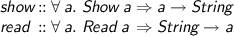
Resolving Type Class Ambiguity. Suppose a programmer wished to normalize the representation of expression text by running it through a parser and then pretty printer. The ${{{\textsf {\textit{normalize}}}}}$ function below maps the string to , resolving precedence and making the meaning clear.⁵

However, the designer of this function cannot make it polymorphic in a straightforward way. Adding a polymorphic type signature results in an ambiguous type, which GHC rightly rejects, as it cannot infer the instantiation for ${{{\textsf {\textit{a}}}}}$ at call sites.

Instead, the programmer must add a ${{{\textsf {\textit{Proxy}}}}}$ argument, which is never evaluated, to allow clients of this polymorphic function to specify the parser and pretty-printer to use

With visible type application, we can write these two functions more directly:⁶

Although the ${{{\textsf {\textit{show}}}}}$/${{{\textsf {\textit{read}}}}}$ ambiguity is somewhat contrived, proxies are indeed useful in more sophisticated APIs. For example, suppose a library designer would like to allow users to choose the representation of an internal data structure to best meet the needs of their application. If the type of that data structure is not included in the input and output types of the API, then a ${{{\textsf {\textit{Proxy}}}}}$ argument is a way to give this control to clients.⁷

Other Examples. More practical examples of the need for visible type application require a fair amount of build-up to motivate the need for the intricate types involved. We have included two larger examples in the extended version [12]. One builds from recent work on deferring constraints until runtime [2] and the other on translating a dependently typed program from Agda [16] into Haskell.

3 Our Approach to Visible Type Application

Visible type application seems like a straightforward extension, but adding this feature – both to GHC and to the HM type system that it is based on – turned out to be more difficult and interesting than we first anticipated. In particular, we encountered two significant questions.

3.1 Just What are the Type Parameters?

The first problem is that it is not always clear what the type parameters to a polymorphic function are!

One aspect of the HM type system is that it permits expressions to be given multiple types. For example, the identity function for pairs,

can be assigned any of the following most general types:

All of these types are principal; no type above is more general than any other. However, the type of the expression,

is very different depending on which “equivalent” type is chosen for ${{{\textsf {\textit{pid}}}}}$:

Of course, there are ad hoc mechanisms for resolving this ambiguity. We could try to designate one of the above types (1–3) as the real principal type for ${{{\textsf {\textit{pid}}}}}$, perhaps by disallowing the quantification of unused variables (ruling out type 3 above) and by enforcing an ordering on how variables are quantified (preferring type 1 over type 2 above). Our goal would be to make sure that each expression has a unique principal type, with respect to its quantified type variables. However, in the context of the full Haskell language, this strategy fails. There are just too many ways that types that are not $\alpha$-equivalent can be considered equivalent by HM. See Fig. 2 for a list of language features that cause difficulties.

Fig. 2.

Why specified polytypes?

In the end, although it may be possible to resolve all of these ambiguities, we prefer not to. That approach leads to a system that is fragile (a new extension could break the requirement that principal types are unique up to $\alpha$-equivalence), difficult to explain to programmers (who must be able to determine which type is principal) and difficult to reason about.

Our Solution: Specified Polytypes. Our system is designed around the following principle:

Only user-specified type parameters can be instantiated via explicit type applications.

In other words, we allow visible type application to instantiate a polytype only when that type is given by a user annotation. This restriction follows in a long line of work requiring user annotations to support advanced type system features [14, 22, 23]. We refer to variables quantified in type annotations as specified variables, distinct from compiler-generated quantified variables, which we call generalized variables.

There is one nuance to this rule in practice. Haskell allows programming to omit variable quantification, allowing a type signature like

Are these variables specified? We have decided that they are. There is a very easy rule at work here: just order the variables left-to-right as the user wrote them. We thus consider variables from type signatures to be specified, even when not bound by an explicit $\forall$.

3.2 Is Our Extension Compatible with the Rest of the Type System?

We do not want to extend just the type inference algorithm that GHC uses. We would also like to extend its specification, which is rooted in HM. This way, we will have a concise description (and better understanding) of what programs type check, and a simple way to reason about the properties of the type system.

Our first attempt to add type application to GHC was based on our understanding of Algorithm $\mathcal {W}$, the standard algorithm for HM type inference. This algorithm instantiates polymorphic functions only at occurrences of variables. So, it seems that the only new form we need to allow is a visible type right after variable occurrences:

However, this extension is not very robust to code refactoring. For example, it is not closed under substitution. If type application is only allowed at variables, then we cannot substitute for this variable and expect the code to still type check. Therefore our algorithm should allow visible type applications at other expression forms. But where else makes sense?

For example, it seems sensible to allow a type instantiation is after a polymorphic type annotation (such an annotation certainly specifies the type of the expression):

Likewise, we should also allow a visible instantiation after a ${{\mathbf {\mathsf{{let}}}}}$ to enable refactoring:⁸

However, how do we know that we have identified all sites where visible type applications should be allowed? Furthermore, we may have identified them all for core HM, but what happens when we go to the full language of GHC, which includes features that may expose new potential sites?

One way to think about this issue in a principled way is to develop a compositional specification of the type system, which allows type application for any expression that can be assigned a polytype. Then, if our algorithm is complete with respect to this specification, we will know that we have allowed type applications in all of the appropriate places. This specification is itself useful in its own right, as we will have a concise description (and better understanding) of what programs type check and a simple way to reason about the properties of the type system.

Once we started thinking of specifications, we found that Algorithm $\mathcal {W}$ could not be matched up with the compositional specification that we wanted. That led us to reconsider our algorithm and develop a new approach to HM type inference.

Our Solution: Lazy Instantiation for Specified Polytypes. Our new type inference algorithm, which we call Algorithm $\mathcal {V}$, is based on the following design principle:

Delay instantiation of “specified” type parameters until absolutely necessary.

Although Algorithm $\mathcal {W}$ instantiates all polytypes immediately, it need not do so. In fact, it is possible to develop a sound and complete alternative implementation of the HM type system that does not do this immediate instantiation. Instead, instantiation is done only on demand, such as when a polymorphic function is applied to arguments. Lazy instantiation has been used in (non-HM) type inference before [10] and may be folklore; however this work contains the first proof that it can be used to implement the HM type system.

In the next section, we give this algorithm a simple specification, presented as a small extension of HM’s existing declarative specification. We then continue with a syntax-directed account of the type system, characterizing where lazy instantiations actually must occur during type checking.

4 HM with Visible Type Application

To make our ideas precise, we next review the declarative specification of the HM type system [7, 13, 18] (which we call System HM), and then show how to extend this specification with visible type arguments.

4.1 System HM

The grammar of System HM is shown in Fig. 3. The expression language comprises the Curry-style typed $\lambda$-calculus with the addition of numeric literals (of type ${{{\textsf {\textit{Int}}}}}$) and ${{\mathbf {\mathsf{{let}}}}}$-expressions. Monotypes are as usual, but we diverge from standard notation in type schemes as they quantify over a possibly-empty set of type variables. Here, we write these type variables in braces to emphasize that they should be considered order-independent. We sometimes write $\tau$ for the type scheme $\forall \{ \, \}.\, \tau$ with an empty set of quantified variables and write $\forall \{ a \}.\, \forall \{ \overline{ b } \}.\, \tau$ to mean $\forall \{ a , \overline{ b } \}.\, \tau$. Here – and throughout this paper – we liberally use the Barendregt convention that bound variables are always distinct from free variables.

Fig. 3.

Grammars for Systems HM and HMV

Fig. 4.

Typing rules for Systems HM and HMV

The declarative typing rules for System HM appear in Fig. 4. (The figure also includes the definition for our extended system, called System HMV, described in Sect. 4.2.) System HM is not syntax-directed; rules HM_Gen and HM_Sub can apply anywhere.

So that we can better compare this system with others in the paper, we make two changes to the standard HM rules. Neither of these changes are substantial; our version types the same programs as the original.⁹ First, in HM_Let, we allow the type of a ${{\mathbf {\mathsf{{let}}}}}$ expression to be a polytype $\sigma$, instead of restricting it to be a monotype $\tau$. We discuss this change further in Sect. 5.2. Second, we replace the usual instantiation rule with HM_Sub. This rule allows the type of any expression to be converted to any less general type in one step (as determined by the subsumption relation $\sigma _{{\mathrm {1}}} \mathrel {\le _{\mathsf {hm} } } \sigma _{{\mathrm {2}}}$). Note that in rule HM_InstG the lists of variables $\overline{ a }_{{\mathrm {1}}}$ and $\overline{ a }_{{\mathrm {2}}}$ need not be the same length.

4.2 System HMV: HM with Visible Types

Fig. 5.

Examples of HMV subsumption relation

System HMV is an extension of System HM, adding visible type application. A key detail in its design is its separation of specified type variables from those arising from generalization, as initially explored in Sect. 3.1. Types may be generalized at any time in HMV, quantifying over a variable free in a type but not free in the typing context. The type variable generalized in this manner is not specified, as the generalization takes place absent any direction from the programmer. By contrast, a type variable mentioned in a type annotation is specified, precisely because it is written in the program text.

The grammar of System HMV appears in Fig. 3. The type language is enhanced with a new intermediate form $\upsilon$ that quantifies over an ordered list of type variables. (We sometimes write $\forall a .\, \forall b .\, \tau$ as $\forall a , b .\, \tau$.) This form sits between type schemes and monotypes; $\sigma$s contain $\upsilon$s, which then contain $\tau$s.¹⁰ Thus the full form of a type scheme $\sigma$ can be written as $\forall \{ \overline{ a } \}, \overline{ b } .\, \tau$, including both a set of generalized variables $\{\overline{ a }\}$ and a list of specified variables $\overline{ b }$. Note that order never matters for generalized variables (they are in a set) while order does certainly matter for specified variables (the list specifies their order). We say that $\upsilon$ is the metavariable for specified polytypes , distinct from type schemes $\sigma$.

Expressions in HMV include two new forms: $e \, \text {@}\tau$ instantiates a specified type variable with a monotype $\tau$, while $( \Lambda \overline{ a } . e : \upsilon )$ allows us to annotate an expression with its type, potentially binding scoped type variables if the type is polymorphic. Requiring a type annotation in concert with scoped type variable binding ensures that the order of quantification is specified: the type annotation is a specified polytype $\upsilon$. We do not allow annotation by type schemes $\sigma$: if the user writes the type, all quantified variables are considered specified.

Typing contexts $\varGamma$ in HMV are enhanced with the ability to store type variables. This feature is used to implement scoped type variables, where the type variables $\overline{ a }$, bound in $\Lambda \overline{ a }. e$, are available for use in types occurring within $e$.

Typing Rules. The type system of HMV includes all of the rules of HM plus the new rules and relation shown at the bottom of Fig. 4. The HMV rules inherited from System HM are modified to recur back to System HMV relations: in effect, replace all $\mathsf {hm}$ subscripts with $\mathsf {hmv}$ subscripts. Note, in particular, rule HM_Sub; in System HMV, this rule refers to the $\sigma _{{\mathrm {1}}} \mathrel {\le _{\mathsf {hmv} } } \sigma _{{\mathrm {2}}}$ relation, described below.

The most important addition to this type system is HMV_TApp, which enables visible type application when the type of the expression is quantified over a specified type variable.

A type annotation $( \Lambda \overline{ a } . e : \upsilon )$, typed with HMV_Annot, allows an expression to be assigned a specified polytype . We require the specified polytype to have the form $\forall \overline{ a } , \overline{ b } .\, \tau$; that is, a prefix of the specified polytype ’s quantified variables must be the type variables scoped in the expression.¹¹ The inner expression $e$ is then checked at type $\tau$, with the type variables $\overline{ a }$ (but not the $\overline{ b }$) in scope. Types that appear in expressions (such as in type annotations and explicit type applications) may mention only type variables that are currently in scope.

Of course, in the premise, the variables $\overline{ a }$ and $\overline{ b }$ may appear in $\tau$. We call such variables skolems and say that skolemizing $\upsilon$ yields $\tau$. In effect, these variables form new type constants when type-checking $e$. When the expression $e$ has type $\tau$, we know that $e$ cannot make any assumptions about the skolems $\overline{ a } , \overline{ b }$, so we can assign $e$ the type $\forall \overline{ a } , \overline{ b } .\, \tau$. This is, in effect, specified generalization.

The relation $\sigma _{{\mathrm {1}}} \mathrel {\le _{\mathsf {hmv} } } \sigma _{{\mathrm {2}}}$ (Fig. 4) implements subsumption for System HMV. The intuition is that, if $\sigma _{{\mathrm {1}}} \mathrel {\le _{\mathsf {hmv} } } \sigma _{{\mathrm {2}}}$, then an expression of type $\sigma _{{\mathrm {1}}}$ can be used wherever one of type $\sigma _{{\mathrm {2}}}$ is expected. For type schemes, the standard notion of $\sigma _{{\mathrm {1}}}$ being a more general type than $\sigma _{{\mathrm {2}}}$ is sufficient. However for specified polytypes, we must be more cautious.

Suppose an expression $x \, \text {@}\tau _{{\mathrm {1}}} \, \text {@}\tau _{{\mathrm {2}}}$ type checks, where $x$ has type $\forall a , b .\, \upsilon _{{\mathrm {1}}}$. The subsumption rule means that we can arbitrarily change the type of $x$ to some $\upsilon$, as long as $\upsilon \mathrel {\le _{\mathsf {hmv} } } \forall a , b .\, \upsilon _{{\mathrm {1}}}$. Therefore, $\upsilon$ must be of the form $\forall a , b .\, \upsilon _{{\mathrm {2}}}$ so that $x \, \text {@}\tau _{{\mathrm {1}}} \, \text {@}\tau _{{\mathrm {2}}}$ will continue to instantiate $a$ with $\tau _{{\mathrm {1}}}$ and $b$ with $\tau _{{\mathrm {2}}}$. Accordingly, we cannot, say, allow subsumption to reorder specified variables.

However, it is safe to allow some instantiation of specified variables as part of subsumption, as in rule HMV_InstS. Examine this rule closely: it instantiates variables from the right. This odd-looking design choice is critical. Continuing the example above, $\upsilon$ could also be of the form $\forall a , b , c .\, \upsilon _{{\mathrm {3}}}$. In this case, the additional specified variable $c$ causes no trouble – it need not be instantiated by a visible application. But we cannot allow instantiation left-to-right as that would allow the visible type arguments to skip instantiating $a$ or $b$.

Further examples illustrating $\, \mathrel {\le _{\mathsf {hmv} } } \,$ appear in Fig. 5.

4.3 Properties of System HMV

We wish System HMV to be a conservative extension of System HM. That is, any expression that is well-typed in HM should remain well-typed in HMV, and any expression not well-typed in HM (but written in the HM subset of HMV) should also not be well-typed in HMV.

Lemma 1

(Conservative Extension for HMV). Suppose $\varGamma$ and $e$ are both expressible in HM; that is, they do not include any type instantiations, type annotations, scoped type variables, or specified polytypes. Then, if and only if .

This property follows directly from the definition of HMV as an extension of HM. Note, in particular, that no HM typing rule is changed in HMV and that the $\, \mathrel {\le _{\mathsf {hmv} } } \,$ relation contains $\, \mathrel {\le _{\mathsf {hm} } } \,$; furthermore, the new rules all require constructs not found in HM.

We also wish to know that making generalized variables into specified variables does not disrupt types:

Lemma 2

(Extra knowledge is harmless). If , then .

This property follows directly from the context generalization lemma below, noting that $\forall \overline{ a } .\, \tau \mathrel {\le _{\mathsf {hmv} } } \forall \{ \overline{ a } \}.\, \tau$.

Lemma 3

(Context generalization for HMV). If , then .

This lemma is proved in the extended version [12].

In practical terms, Lemma 2 means that if an expression contains ${{\mathbf {\mathsf{{let}}}}} \, x = e_{{\mathrm {1}}} \, {{\mathbf {\mathsf{{in}}}}} \, e_{{\mathrm {2}}}$, and the programmer figures out the type assigned to $x$ (say, $\forall \{ \overline{ a } \}.\, \tau$) and then includes that type in an annotation (as ${{\mathbf {\mathsf{{let}}}}} \, x = ( e_{{\mathrm {1}}} : \forall \overline{ a } .\, \tau ) \, {{\mathbf {\mathsf{{in}}}}} \, e_{{\mathrm {2}}}$), the outer expression’s type does not then change.

However, note that, by design, context generalization is not as flexible for specified polytypes as it is for type schemes. In other words, suppose the following expression type-checks.

The programmer cannot then replace the type annotation with the type $\forall \;{{{\textsf {\textit{a}}}}}.\;{{{\textsf {\textit{a}}}}}\rightarrow {{{\textsf {\textit{a}}}}}$, because ${{{\textsf {\textit{x}}}}}$ may be used with visible type applications. This behavior may be surprising, but it follows directly from the fact that $\forall \;{{{\textsf {\textit{a}}}}}.\;{{{\textsf {\textit{a}}}}}\rightarrow {{{\textsf {\textit{a}}}}} \mathrel {\not \le _{\mathsf {hmv} } } \forall \;{{{\textsf {\textit{a}}}}}\;{{{\textsf {\textit{b}}}}}.\;({{{\textsf {\textit{a}}}}},{{{\textsf {\textit{b}}}}})\rightarrow ({{{\textsf {\textit{a}}}}},{{{\textsf {\textit{b}}}}})$.

Finally, we would also like to show that HMV retains the principal types property, defined with respect to the enhanced subsumption relation $\sigma _{{\mathrm {1}}} \mathrel {\le _{\mathsf {hmv} } } \sigma _{{\mathrm {2}}}$.

Theorem 4

(Principal types for HMV). For all terms $e$ well-typed in a context $\varGamma$, there exists a type scheme $\sigma _{\mathrm {p} }$ such that and, for all $\sigma$ such that .

Before we can prove this, we first must show how to extend HM’s type inference algorithm (Algorithm $\mathcal {W}$  [8]) to include visible type application. Once we do so, we can prove that this new algorithm always computes principal types.

5 Syntax-Directed Versions of HM and HMV

The type systems in the previous section declare when programs are well-formed, but they are fairly far removed from an algorithm. In particular, the rules HM_Gen and HM_Sub can appear at any point in a typing derivation.

Fig. 6.

Syntax-directed version of the HM type system

5.1 System C

We can explain the HM type system in a more algorithmic manner by using a syntax-directed specification, called System C, in Fig. 6. This version of the type system, derived from Clément et al. [5], clarifies exactly where generalization and instantiation occur during type checking. Notably, instantiation occurs only at the usage of a variable, and generalization occurs only at a ${{\mathbf {\mathsf{{let}}}}}$-binding. These rules are syntax-directed because the conclusion of each rule in the main judgment is syntactically distinct. Thus, from the shape of an expression, we can determine the shape of its typing derivation.

However, the judgment is still not quite an algorithm: it makes non-deterministic guesses. For example, in the rule C_Abs, the type $\tau _{{\mathrm {1}}}$ is guessed; there is no indication in the expression what the choice for $\tau _{{\mathrm {1}}}$ should be. The advantage of studying a syntax-directed system such as System C is that doing so separates concerns: System C fixes the structure of the typing derivation (and of any implementation) while leaving monotype-guessing as a separate problem. Algorithm $\mathcal {W}$ deduces the monotypes via unification, but a constraint-based approach [25, 27] would also work.

5.2 System V: Syntax-Directed Visible Types

Just as System C is a syntax-directed version of HM, we can also define System V, a syntax-directed version of HMV (Fig. 7). However, although we could define HMV by a small addition to HM (two new rules, plus subsumption), the difference between System C and System V is more significant.

Fig. 7.

Typing rules for System V

Like System C, System V uses multiple judgments to restrict where generalization and instantiation can occur. In particular, the system allows an expression to have a type scheme only as a result of generalization (using the judgment ). Generalization is, once again, available only in ${{\mathbf {\mathsf{{let}}}}}$-expressions.

However, the main difference that enables visible type annotation is the separation of the main typing judgment into two: and . The key idea is that, sometimes, we need to be lazy about instantiating specified type variables so that the programmer has a chance to add a visible instantiation. Therefore, the system splits the rules into a judgment that requires $e$ to have a monotype, and those in that can retain specified quantification.

The first set of rules in Fig. 7, as in System C, infers a monotype for the expression. The premises of the rule V_Abs uses this same judgment, for example, to require that the body of an abstraction have a monotype. All expressions can be assigned a monotype; if the first three rules do not apply, the last rule V_InstS infers a polytype instead, then instantiates it to yield a monotype. Because implicit instantiation happens all at once in this rule, we do not need to worry about instantiating specified variables out of order, as we did in System HMV.

The second set of rules (the judgment) allows $e$ to be assigned a specified polytype. Note that the premise of rule V_TApp uses this judgment.

Rule V_Var is like rule C_Var: both look up a variable in the environment and instantiate its generalized quantified variables. The difference is that C_Var’s types can contain only generalized variables; System V’s types can have specified variables after the generalized ones. Yet we instantiate only the generalized ones in the V_Var rule, lazily preserving the specified ones.

Rule V_Let is likewise similar to C_Let. The only difference is that the result type is not restricted to be a monotype. By putting V_Let in the judgment and returning a specified polytype, we allow the following judgment to hold:

The expression above would be ill-typed in a system that restricted the result of a ${{\mathbf {\mathsf{{let}}}}}$-expression to be a monotype. It is for this reason that we altered System HM to include a polytype in its HM_Let rule, for consistency with HMV.

Rule V_Annot is identical to rule HMV_Annot. It uses the judgment in its premise to force instantiation of all quantified type variables before regeneralizing to the specified polytype $\upsilon$. In this way, the V_Annot rule is effectively able to reorder specified variables. Here, reordering is acceptable, precisely because it is user-directed.

Finally, if an expression form cannot yield a specified polytype, rule V_Mono delegates to to find a monotype for the expression.

5.3 Relating System V to System HMV

Systems HMV and V are equivalent; they type check the same set of expressions. We prove this correspondence using the following two theorems.

Theorem 5

(Soundness of V against HMV)

• 1. If , then .

• 2. If , then .

• 3. If , then .

Theorem 6

(Completeness of V against HMV). If , then there exists $\sigma '$ such that where $\sigma ' \mathrel {\le _{\mathsf {hmv} } } \sigma$.

The proofs of these theorems appear in the extended version [12].

Having established the equivalence of System V with System HMV, we can note that Lemma 2 (“Extra knowledge is harmless”) carries over from HMV to V. This property is quite interesting in the context of System V. It says that a typing context where all type variables are specified admits all the same expressions as one where some type variables are generalized. In System V, however, specified and generalized variables are instantiated via different mechanisms, so this is a powerful theorem indeed.

It is mechanical to go from the statement of System V in Fig. 7 to an algorithm. In the extended version [12], we define Algorithm $\mathcal {V}$ which implements System V, analogous to Algorithm $\mathcal {W}$ which implements System C. We then prove that Algorithm $\mathcal {V}$ is sound and complete with respect to System V and that Algorithm $\mathcal {V}$ finds principal types. Linking the pieces together gives us the proof of the principal types property for System HMV (Theorem 4). Furthermore, Algorithm $\mathcal {V}$ is guaranteed to terminate, yielding this theorem:

Theorem 7

Type-checking System V is decidable.

6 Higher-Rank Type Systems

We now extend the design of System HMV to include higher-rank polymorphism [17]. This extension allows function parameters to be used at multiple types. Incorporating this extension is actually quite straightforward. We include this extension to show that our framework for visible type application is indeed easy to extend – the syntax-directed system we study in this section is essentially a merge of System V and the bidirectional system from our previous work [23]. This system is also the basis for our implementation in GHC.

As an example, the following function does not type check in the vanilla Hindley-Milner type system, assuming ${{{\textsf {\textit{id}}}}}$ has type $\forall \;{{{\textsf {\textit{a}}}}}.\;{{{\textsf {\textit{a}}}}}\rightarrow {{{\textsf {\textit{a}}}}}$.

Yet, with the RankNTypes language extension and the following type annotation, GHC is happy to accept

Visible type application means that higher-rank arguments can also be explicitly instantiated. For example, we can instantiate lambda-bound identifiers:

Higher-rank types also mean that visible instantiations can occur after other arguments are passed to a function. For example, consider this alternative type for the ${{{\textsf {\textit{pair}}}}}$ function:

If ${{{\textsf {\textit{pair}}}}}$ has this type, we can instantiate ${{{\textsf {\textit{b}}}}}$ after providing the first component for the pair, thus:

In the rest of this section, we provide the technical details of these language features and discuss their interactions. In contrast to the presentation above, we present the syntax-directed higher-rank system first. We do so for two reasons: understanding a bidirectional system requires thinking about syntax, and thus the syntax-directed system seems easier to understand; and we view the declarative system as an expression of properties – or a set a metatheorems – about the higher-rank type system.

6.1 System SB: Syntax-Directed Bidirectional Type Checking

Fig. 8.

Syntax-directed bidirectional type system

Fig. 9.

Higher-rank subsumption relations

Figures 8 and 9 show System SB, the higher-rank, bidirectional analogue of System V, supporting predicative higher-rank polymorphism and visible type application.

This system shares the same expression language of Systems HMV and V, retaining visible type application and type annotations. However, types in System SB may have non-prenex quantification. The body of a specified polytype $\upsilon$ is now a phi-type $\phi$: a type that has no top-level quantification but may have quantification to the left or to the right of arrows. Note also that these inner quantified types are $\upsilon$s, not $\sigma$s. In other words, non-prenex quantification is over only specified variables, never generalized ones. As we will see, inner quantified types are introduced only by user annotation, and thus there is no way the system could produce an inner type scheme, even if the syntactic restriction were not in place.

The grammar also defines rho-types $\rho$, which also have no top-level quantification, but do allow inner quantification to the left of arrows. We convert specified polytypes (which may quantify to the right of arrows) to corresponding rho-types by means of the $prenex$ operation, which appears in Fig. 9.

System SB is defined by five mutually recursive judgments: , , and are synthesis judgments, producing the type as an output; and are checking judgments, requiring the type as an input.

Type Synthesis. The synthesis judgments are very similar to the judgments from System V, ignoring direction arrows. The differences stem from the non-prenex quantification allowed in SB. The level of similarity is unsurprising, as the previous systems essentially all work only in synthesis mode; they derive a type given an expression. The novelty of a bidirectional system is its ability to propagate information about specified polytypes toward the leaves of an expression.

Type Checking. Rule SB_DAbs is what makes the system higher-rank. The checking judgment pushes in a rho-type, with no top-level quantification. Thus, SB_DAbs can recognize an arrow type $\upsilon _{{\mathrm {1}}} \rightarrow \rho _{{\mathrm {2}}}$. Propagating this type into an expression $\lambda x .\, e$, SB_DAbs uses the type $\upsilon _{{\mathrm {1}}}$ as $x$’s type when checking $e$. This is the only place in system SB where a lambda-term can abstract over a variable with a polymorphic type. Note that the synthesis rule SB_Abs uses a monotype for the type of x.¹²

Rule SB_Infer mediates between the checking and synthesis judgments. When no checking rule applies, we synthesize a type and then check it according to the $\le _{\mathsf {dsk} }$ deep skolemization relation, taken directly from previous work and shown in Fig. 9. For brevity, we do not explain the details of this relation here, instead referring readers to Peyton Jones et al. [23, Sect. 4.6] for much deeper discussion. However, we note that there is a design choice to be made here; we could have also used Odersky–Läufer’s slightly less expressive higher-rank subsumption relation [21] instead. We present the system with deep skolemization for backwards compatibility with GHC. See the extended version [12] for a discussion of this alternative.

The entry point into the type checking judgments is through the judgment. This judgment has just one rule, SB_DeepSkol. The rule skolemizes all type variables appearing at the top-level and to the right of arrows. Skolemizing here is necessary to expose a rho-type to the judgment, so that rule SB_DAbs can fire.¹³ The reason this rule requires deep skolemization instead of top-level skolemization is subtle, but this choice is not due to visible type application or lazy instantiation; the same choice is made in prior work [23, rulegen2 of Fig. 8]. We refer readers to the extended version [12] for the details.

Fig. 10.

System B

6.2 System B: Declarative Specification

Figure 10 shows the typing rules of System B, a declarative system that accepts the same programs as System SB. This declarative type system itself is a novel contribution of this work. (The systems presented in related work [10, 21, 23] are more similar to SB than to B.)

Although System B is bidirectional, it is also declarative. In particular, the use of generalization (B_Gen), subsumption (B_Sub), skolemization (B_Skol), and mode switching (B_Infer), can happen arbitrarily in a typing derivation. Understanding what expressions are well-typed does not require knowing precisely when these operations take place.

The subsumption rule (B_Sub) in the synthesis judgment corresponds to HMV_Sub from HMV. However, the novel subsumption relation $\, \mathrel {\le _{\mathsf {b} } } \,$ used by this rule, shown at the top of Fig. 9, is different from the $\le _{\mathsf {dsk} }$ deep skolemization relation used in System SB. This $\sigma _{{\mathrm {1}}} \mathrel {\le _{\mathsf {b} } } \sigma _{{\mathrm {2}}}$ judgment extends the action of $\, \mathrel {\le _{\mathsf {hmv} } } \,$ to higher-rank types: in particular, it allows subsumption for generalized type variables (which can be quantified only at the top level) and instantiation (only) for specified type variables. We could say that this judgment enables inner instantiation because instantiations are not restricted to top level. See also the examples at the bottom of Fig. 9.

In contrast, rule B_Infer (in the checking judgment) uses the stronger of the two subsumption relations $\le _{\mathsf {dsk} }$. This rule appears at precisely the spot in the derivation where a specified type from synthesis mode meets the specified type from checking mode. The relation $\le _{\mathsf {dsk} }$ subsumes $\, \mathrel {\le _{\mathsf {b} } } \,$; that is, $\sigma _{{\mathrm {1}}} \mathrel {\le _{\mathsf {b} } } \upsilon _{{\mathrm {2}}}$ implies $\sigma _{{\mathrm {1}}} \le _{\mathsf {dsk} } \upsilon _{{\mathrm {2}}}$.

Properties of System B and SB. We can show that Systems SB and B admit the same expressions.

Lemma 8

(Soundness of System SB)

• 1. If then .

• 2. If then .

• 3. If then .

• 4. If then .

• 5. If then .

Lemma 9

(Completeness of System SB)

• 1. If then where $\sigma ' \mathrel {\le _{\mathsf {b} } } \sigma$.

• 2. If then .

What is the role of System B? In our experience, programmers tend to prefer the syntax-directed presentation of the system because that version is more algorithmic. As a result, it can be easier to understand why a program type checks (or doesn’t) by reasoning about System SB.

However, the fact that System B is sound and complete with respect to System SB provides properties that we can use to reason about SB. The main difference between the two is that System B divides subsumption into two different relations. The weaker $\, \mathrel {\le _{\mathsf {b} } } \,$ can be used at any time during synthesis, but it can only instantiate (but not generalize) specified variables. The stronger $\le _{\mathsf {dsk} }$ is used at only the check/synthesis boundary but can generalize and reorder specified variables.

The connection between the two systems tells us that B_Sub is admissible for SB. As a result, when refactoring code, we need not worry about precisely where a type is instantiated, as we see here that instantiation need not be determined syntactically.

Likewise, the proof also shows that System B (and System SB) is flexible with respect to the instantiation relation $\, \mathrel {\le _{\mathsf {b} } } \,$ in the context. As in System HMV, this result implies that making generalized variables into specified variables does not disrupt types.

Lemma 10

(Context Generalization). Suppose $\varGamma ' \mathrel {\le _{\mathsf {b} } } \varGamma$.

• 1. If then there exists $\sigma ' \mathrel {\le _{\mathsf {b} } } \sigma$ such that .

• 2. If and $\upsilon \mathrel {\le _{\mathsf {b} } } \upsilon '$ then .

Proofs of these properties appear in the extended version [12].

6.3 Integrating Visible Type Application with GHC

System SB is the direct inspiration for the type-checking algorithm used in our version of GHC enhanced with visible type application. It is remarkably straightforward to implement the system described here within GHC; accounting for the behavior around imported functions (Sect. 3.1) was the hardest part. The other interactions (the difference between this paper’s scoped type variables and GHC’s, how specified type variables work with type classes, etc.) are generally uninteresting; see the extended version [12] for further comments.

One pleasing synergy between visible type application and GHC concerns GHC’s recent partial type signature feature [29]. This feature allows wildcards, written with an underscore, to appear in types; GHC infers the correct replacement for the wildcard. These work well in visible type applications, allowing the user to write as a visible type argument where GHC can infer the argument. For example, if ${{{\textsf {\textit{f}}}}}$ has type $\forall \;{{{\textsf {\textit{a}}}}}\;{{{\textsf {\textit{b}}}}}.\;{{{\textsf {\textit{a}}}}}\rightarrow {{{\textsf {\textit{b}}}}}\rightarrow ({{{\textsf {\textit{a}}}}},{{{\textsf {\textit{b}}}}})$, then we can write to let GHC infer that ${{{\textsf {\textit{a}}}}}$ should be ${{{\textsf {\textit{Bool}}}}}$ but to visibly instantiate ${{{\textsf {\textit{b}}}}}$ to be . Getting partial type signatures to work in the new context of visible type applications required nothing more than hooking up the pieces.

7 Related Work and Conclusions

Explicit Type Arguments. The F# language [26] permits explicit type arguments in function applications and method invocations. These explicit arguments, typically mandatory, are used to resolve ambiguity in type-dependent operations. However, the properties of this feature have not been studied.

Implicit Arguments in Dependently-Typed Languages. Languages such as Coq [6], Agda [20], Idris [1] and Twelf [24] are not based on the HM type system, so their designs differ from Systems HMV and B. However, they do support invisible arguments. In these languages, an invisible argument is not necessarily a type; it could be any argument that can be inferred by the type checker.

Coq, Agda, and Idris require all quantification, including that for invisible arguments, to be specified by the user. These languages do not support generalization, i.e., automatically determining that an expression should quantify over an invisible argument (in addition to any visible ones). They differ in how they specify the visibility of arguments, yet all of them provide the ability to override an invisibility specification and provide such arguments visibly. These languages also provide a facility for named invisible arguments, allowing users to specify argument values by name instead of by position. This choice means that $\alpha$-equivalent types are no longer fully interchangeable. Though we have not studied this possibility deeply, we conjecture that formally specifying a named-argument system would encounter many of the same subtleties (in particular, requiring two different subsumption relations in the metatheory) that we encountered with positional arguments.

Twelf, on the other hand, supports invisible arguments via generalization and visible arguments via specification. Although it is easy to convert between the two versions, there is no way to visibly provide an invisible argument as we have done. Instead, the user must rely on type annotations to control instantiations.

Specified vs. Generalized Variables. Dreyer and Blume’s work on specifying ML’s type system and inference algorithm in the presence of modules [9] introduces a separation of (what we call) specified and generalized variables. Their work focuses on the type parameters to ML functors, finding inconsistencies between the ML language specification and implementations. They conclude that the ML specification as written is hard to implement and propose a new one. Their work includes a type system that allows functors to have invisible arguments alongside their visible ones. This specification is easier to implement, as they demonstrate.

Their work has similarities to ours in the separation of classes of variables and the need to alter the specification to make type inference reasonable. Interestingly, they come from the opposite direction from ours, adding invisible arguments in a place where arguments previously were all visible. However, despite these surface similarities, we have not found a deeper connection between our work and theirs.

Predicative, Higher-Rank Type Systems. As we have already indicated, Systems B and SB are directly inspired by GHC’s design for higher-rank types [23]. However, in this work we have redesigned the algorithm to use lazy instantiation and have made a distinction between specified polytypes and generalized polytypes. Furthermore, we have pushed the design further, providing a declarative specification for the type system.

Our work is also closely related to recent work on using a bidirectional type system for higher-rank polymorphism by Dunfield and Krishnaswami [10], called DK below. The closest relationship is between their declarative system (Fig. 4 in their paper) and our System SB (Fig. 8). The most significant difference is that the DK system never generalizes. All polymorphic types in their system are specified; functions must have a type annotation to be polymorphic. Consequently, DK uses a different algorithm for type checking than the one proposed in this work. Nevertheless, it defers instantiations of specified polymorphism, like our algorithm.

Our relation $\le _{\mathsf {dsk} }$, which requires two specified polytypes, is similar to the DK subsumption relation. The DK version is slightly weaker as it does not use deep skolemization; but that difference is not important in this context. Another minor difference is that System SB uses the judgment to syntactically guide instantiation whereas the the DK system uses a separate application judgment form. System B – and the metatheory of System SB – also includes implicit subsumption $\, \mathrel {\le _{\mathsf {b} } } \,$, which does not have an analogue in the DK system. A more extended comparison with the DK system appears in the extended version [12].

Conclusion. This work extends the HM type system with visible type application, while maintaining important properties of that system that make it useful for functional programmers. Our extension is fully backwards compatible with previous versions of GHC. It retains the principal types property, leading to robustness during refactoring. At the same time, our new systems come with simple, compositional specifications.

While we have incorporated visible type application with all existing features of GHC, we do not plan to stop there. We hope that our mix of specified polytypes and type schemes will become a basis for additional type system extensions, such as impredicative types, type-level lambdas, and dependent types.

References

Brady, E.: Idris, a general-purpose dependently typed programming language: design and implementation. J. Funct. Prog. 23, 552–593 (2013)
Buiras, P., Vytiniotis, D., Alejandro Russo, H.: Mixing static and dynamic typing for information-flow control in Haskell. In: International Conference on Functional Programming, ICFP 2015. ACM (2015)
Chakravarty, M.M.T., Keller, G., Peyton Jones, S.: Associated type synonyms. In: International Conference on Functional Programming, ICFP 2005. ACM (2005)
Chakravarty, M.M.T., Keller, G., Peyton Jones, S., Marlow, S.: Associated types with class. In: ACM SIGPLAN-SIGACT Symposium on Principles of Programming Languages (2005)
Clément, D., Despeyroux, T., Kahn, G., Joëlle Despeyroux, A.: simple applicative language : Mini-ML. In: Conference on LISP and Functional Programming, LFP 1986. ACM (1986)
Coq development team. The Coq proof assistant reference manual. LogiCal Project. Version 8.0 (2004). http://coq.inria.fr
Damas, L.: Type Assignment in Programming Languages. PhD thesis, University of Edinburgh (1985)
Damas, L., Milner, R.: Principal type-schemes for functional programs. In: Symposium on Principles of Programming Languages, POPL 1982. ACM (1982)
Dreyer, D., Blume, M.: Principal type schemes for modular programs. In: De Nicola, R. (ed.) ESOP 2007. LNCS, vol. 4421, pp. 441–457. Springer, Heidelberg (2007)
Dunfield, J., Krishnaswami, N.R.: Complete and easy bidirectional typechecking for higher-rank polymorphism. In: International Conference on Functional Programming, ICFP 2013. ACM (2013)
Eisenberg, R.A., Vytiniotis, D., Peyton Jones, S., Weirich, S.: Closed type families with overlapping equations. In: Principles of Programming Languages, POPL 2014. ACM (2014)
Eisenberg, R.A., Weirich, S., Ahmed, H.: Visible type application (extended version) (2015). http://www.seas.upenn.edu/~sweirich/papers/type-app-extended.pdf
Hindley, J.R.: The principal type-scheme of an object in combinatory logic. Trans. Am. Math. Soc. 146, 29–60 (1969)
Le Botlan, D., Rémy, D.: \({\rm ML}^F\): Raising ML to the power of System F. In: International Conference on Functional Programming. ACM (2003)
Marlow, S. (ed.): Haskell language report (2010)
McBride, C.: Agda-curious? Keynote. In: ICFP 2012 (2012)
McCracken, N.: The typechecking of programs with implicit type structure. In: Kahn, G., MacQueen, D.B., Plotkin, G. (eds.) Semantics of Data Types. LNCS, vol. 173, pp. 301–315. Springer, Heidelberg (1984)
Milner, R.: A theory of type polymorphism in programming. J. Comput. Syst. Sci. 17, 348–375 (1978)
Miquel, A.: The implicit calculus of constructions. In: Abramsky, S. (ed.) TLCA 2001. LNCS, vol. 2044, pp. 344–359. Springer, Heidelberg (2001)
Norell, U.: Towards a practical programming language based on dependent type theory. PhD thesis, Department of Computer Science and Engineering, Chalmers University of Technology, SE-412 96 Göteborg, Sweden, September 2007
Odersky, M., Läufer, K.: Putting type annotations to work. In: Symposium on Principles of Programming Languages, POPL 1996. ACM (1996)
Peyton Jones, S., Vytiniotis, D., Weirich, S., Washburn, G.: Simple unification-based type inference for GADTs. In: International Conference on Functional Programming, ICFP 2006. ACM (2006)
Peyton Jones, S., Vytiniotis, D., Weirich, S., Shields, M.: Practical type inference for arbitrary-rank types. J. Func. Program. 17(1), 1–82 (2007)
Pfenning, F., Schürmann, C.: System description: Twelf - a meta-logical framework for deductive systems. In: Ganzinger, H. (ed.) CADE 1999. LNCS (LNAI), vol. 1632, pp. 202–206. Springer, Heidelberg (1999)
Pottier, F., Rémy, D.: The Essence of ML Type Inference. In: Pierce, B.C. (ed.) Advanced Topics in Types and Programming Languages, pp. 387–489. The MIT Press (2005)
Syme, D.: The F# 2.0 Language Specification. Microsoft Research and the Microsoft Developer Division (2012). http://fsharp.org/specs/language-spec/2.0/FSharpSpec-2.0-April-2012.pdf
Vytiniotis, D., Peyton Jones, S., Schrijvers, T., Sulzmann, M.: OutsideIn(X) modular type inference with local assumptions. J. Funct. Program. 21(4–5), 333–412 (2011)
Wadler, P., Blott, S.: How to make ad-hoc polymorphism less ad-hoc. In: POPL, pp. 60–76. ACM (1989)
Winant, T., Devriese, D., Piessens, F., Schrijvers, T.: Partial type signatures for haskell. In: Flatt, M., Guo, H.-F. (eds.) PADL 2014. LNCS, vol. 8324, pp. 17–32. Springer, Heidelberg (2014)
Acknowledgments
Thanks to Simon Peyton Jones, Dimitrios Vytiniotis, Iavor Diatchki, Adam Gundry, Conor McBride, Neel Krishnaswami, and Didier Rémy for helpful discussion and feedback.
Author information
Authors and Affiliations
Corresponding authors
Editor information
Editors and Affiliations
Rights and permissions
Copyright information
© 2016 Springer-Verlag Berlin Heidelberg
About this paper
Cite this paper
Eisenberg, R.A., Weirich, S., Ahmed, H.G. (2016). Visible Type Application. In: Thiemann, P. (eds) Programming Languages and Systems. ESOP 2016. Lecture Notes in Computer Science(), vol 9632. Springer, Berlin, Heidelberg. https://doi.org/10.1007/978-3-662-49498-1_10
Download citation
DOI: https://doi.org/10.1007/978-3-662-49498-1_10
Publisher Name: Springer, Berlin, Heidelberg
Print ISBN: 978-3-662-49497-4
Online ISBN: 978-3-662-49498-1
eBook Packages: Computer ScienceComputer Science (R0)