Trading Plaintext-Awareness for Simulatability to Achieve Chosen Ciphertext Security

Abstract

In PKC 2014, Dachman-Soled showed a construction of a chosen ciphertext (CCA) secure public key encryption (PKE) scheme based on a PKE scheme which simultaneously satisfies a security property called weak simulatability and (standard model) plaintext awareness (sPA1) in the presence of multiple public keys. It is not well-known if plaintext awareness for the multiple keys setting is equivalent to the more familiar notion of that in the single key setting, and it is typically considered that plaintext awareness is a strong security assumption (because to achieve it we have to rely on a “knowledge”-type assumption). In Dachman-Soled’s construction, the underlying PKE scheme needs to be plaintext aware in the presence of $2k+2$ public keys.

The main result in this work is to show that the strength of plaintext awareness required in the Dachman-Soled construction can be somehow “traded” with the strength of a “simulatability” property of other building blocks. Furthermore, we also show that we can “separate” the assumption that a single PKE scheme needs to be both weakly simulatable and plaintext aware in her construction. Specifically, in this paper we show two new constructions of CCA secure key encapsulation mechanisms (KEMs): Our first scheme is based on a KEM which is chosen plaintext (CPA) secure and plaintext aware only under the 2 keys setting, and a PKE scheme satisfying a “slightly stronger” simulatability than weak simulatability, called “trapdoor simulatability” (introduced by Choi et al. ASIACRYPT 2009). Our second scheme is based on a KEM which is 1-bounded CCA secure (Cramer et al. ASIACRYPT 2007) and plaintext aware only in the single key setting, and a trapdoor simulatable PKE scheme. Our results add new recipes for constructing CCA secure PKE/KEM from general assumptions (that are incomparable to those used by Dachman-Soled), and in particular show interesting trade-offs among building blocks with those used in Dachman-Soled’s construction.

1 Introduction

1.1 Background and Motivation

For public key encryption (PKE), security (indistinguishability) against chosen ciphertext attacks (CCA) [23, 46, 49] is nowadays considered as a de-facto standard security notion required in most practical situations/applications in which PKE schemes are used. CCA security is quite important in both practical and theoretical points of view. It implies security against practical attacks (e.g. Bleichenbacher’s attack [8]) and it also implies very strong and useful security notions, such as non-malleability [23] and universal composability [10]. Thus, constructing and understanding CCA secure PKE schemes is one of the central research themes in the area of cryptography. In this paper, we focus on the constructions of CCA secure PKE schemes and its closely related primitive called key encapsulation mechanism (KEM) from general cryptographic assumptions. There have been a number of works that show that several different kinds of cryptographic primitives are sufficient to realize CCA secure PKE/KEM: These include trapdoor permutations [23] (with some enhanced property [27]), identity-based encryption [12] and a weaker primitive called tag-based encryption [32], lossy trapdoor function [48] and related primitives [13, 33, 42, 50, 54], PKE schemes with weaker-than-but-close-to-CCA security [31, 34, 40], positive results on cryptographic obfuscation [38, 52], the combination of a CPA secure PKE scheme and a strong form of hash functions [39], and very recently, the combination of a sender non-committing encryption scheme and a key-dependent-message secure symmetric key encryption (SKE) scheme [41]. (We review more works in Sect. 1.4).

In PKC 2014, Dachman-Soled [18] showed a construction of a CCA secure PKE scheme based on a PKE scheme which simultaneously satisfies a security property called weak simulatability [20, 43] and (standard model) plaintext awareness (sPA1) [5] in the presence of multiple public keys [43], which is based on the earlier work by Myers et al. [43] who showed a construction of a PKE scheme that achieves security slightly weaker than CCA (the so-called cNM-CCA1 security). Plaintext awareness was first introduced by Bellare and Rogaway [7] as a useful notion for showing CCA security of a PKE scheme in the random oracle model [6], and was used in a number of random-oracle-model constructions (e.g. [7, 24, 25, 47]). Bellare and Palacio [5] defined the standard model versions of plaintext awareness.¹ The plaintext awareness notions were further studied by subsequent works (e.g. [20]). The most works on plaintext awareness studied the notions for the single key setting. The extension to the multiple keys setting was first introduced by Myers et al. [43].

We note that it is not well-known or well-studied if plaintext awareness for the multiple keys setting is equivalent to the more familiar notion of plaintext awareness in the single key setting, and it is typically considered that plaintext awareness is a strong security assumption (because to achieve it we have to rely on a “knowledge”-type assumption). In the construction of [18], the underlying PKE scheme needs to be plaintext aware in the presence of $2k+2$ public keys. Our motivation in this work is to clarify whether we can weaken the assumption of plaintext awareness in Dachman-Soled’s construction [18]. As mentioned in [18], a plaintext aware (sPA1) PKE scheme seems almost like a CCA1 secure PKE scheme [46], but it seems not possible to replace the building block PKE scheme in [18] with a CCA1 secure scheme to remove the plaintext awareness. It is currently not known if we can construct a CCA secure PKE scheme only from a CPA secure scheme or even from a CCA1 secure scheme. We believe that studying the possibility of weakening the assumption of plaintext awareness from [18] thus is expected to lead to deepening our knowledge on this topic, and generally contribute to the long line of research on clarifying the minimal general assumption that implies CCA secure PKE.

1.2 Our Contributions

Based on the motivation mentioned above, we study the possibility of weakening the requirements of plaintext awareness used in Dachman-Soled’s construction [18], and come up with new results that show that the strength of plaintext awareness required in [18] can be somehow “traded” with the strength of a “simulatability” property of other building blocks. Furthermore, we also show that we can “separate” the requirement that a single PKE scheme needs to be simultaneously weakly simulatable and plaintext aware, in her construction.

Specifically, in this paper we show two new constructions of CCA secure KEMs (which are given in Sect. 4), based on the assumptions that are incomparable to those used in [18]:

• Our first construction (Sect. 4.1) is based on a KEM which is chosen plaintext (CPA) secure and plaintext aware only under the 2 keys setting², and a PKE scheme satisfying a “slightly stronger” simulatability than weak simulatability, called “trapdoor simulatability” (introduced by Choi et al. [14]). Actually, although we write that it is “slightly stronger”, it is formally incomparable to weak simulatability. For more details, see Sect. 1.3.

• Our second construction (Sect. 4.2) is based on a KEM which is 1-bounded CCA secure [15] and plaintext aware only in the single key setting, and a trapdoor simulatable PKE scheme. We can in fact slightly weaken the requirement of 1-bounded CCA security to CPA security in the presence of one “plaintext-checking” query [1, 47]. We will also show that we can construct a KEM satisfying simultaneously 1-bounded CCA security and plaintext awareness under the single key setting, based on a KEM satisfying CPA security and plaintext awareness under the 2k keys setting, via the recent result by Dodis and Fiore [21, Appendix C].

  One may wonder the meaning of the second construction, because if we use a KEM that is plaintext aware under O(k) keys setting, there is no merit compared to our first construction. We are however considering it to be still meaningful in several aspects, and we refer the reader to Sect. 4.2 for more discussions regarding the second construction.

Note that from CCA secure KEMs, we can immediately obtain full-fledged PKE schemes by using CCA secure SKE [16].

We emphasize that we do not require plaintext awareness and the trapdoor simulatability property to be satisfied by a single building block. This “separation” of the requirements should be contrasted with Dachman-Soled’s construction [18], the building block PKE scheme of which is required to satisfy plaintext awareness and the weak simulatability property simultaneously. We also again emphasize that the assumptions on which both of our constructions are based, are incomparable to those used in [18]. Thus, our results add new recipes for constructing CCA secure PKE/KEM from general assumptions (and thus the assumptions that we use could be new targets that are worth pursuing), and also show interesting trade-offs regarding assumptions with Dachman-Soled’s construction.

1.3 Technical Overview

Assumptions on the Building Blocks. Trapdoor simulatable PKE (TSPKE) [14] is the key building block for our constructions. TSPKE is a weaker (relaxed) version of simulatable PKE that was originally formalized by Damgård and Nielsen [19]. Simulatable PKE admits “oblivious sampling” of both public keys and ciphertexts (i.e. sampling them without knowing the randomness or plaintext) in such a way that honestly generated public keys and ciphertexts can be later convincingly explained that they were generated obliviously. These properties are realized by requiring that the key generation algorithm and the encryption algorithm have their own “oblivious sampling” algorithm and its corresponding “inverting” algorithm (where the inverting algorithm corresponds to the algorithm that “explains” that an honest generated public key (or a ciphertext) is sampled obliviously). The difference between TSPKE and simulatable PKE is whether we allow the “inverting” algorithm to take the randomness (and the plaintext) used by the ordinary algorithms (key generation and encryption algorithms) as input. TSPKE allows to take these inputs, while ordinary simulatable PKE does not, which makes the security property of TSPKE weaker but easier to achieve. For our purpose, we only need even a simplified version of TSPKE than the formalization in [14]: we only require a pair (pk, c) of public key/ciphertext (or, a “transcript”) can be obliviously sampled, but not each of pk and c can be so (which is the formalization in [14]). It was shown [14, 19] that we can realize TSPKE from a number of standard cryptographic assumptions, such as the computational and decisional Diffie-Hellman assumptions, RSA, Factoring, and lattice based assumptions. (For more details, see Sect. 2.2).

On the other hand, a weakly simulatable PKE scheme (used in the constructions in [18, 43]) considers oblivious sampling only for the encryption algorithm. However, the definition of weakly simulatable PKE used in [18, 43] does not allow the inverting algorithms to take the randomness and the plaintext used by the ordinary encryption algorithm. Therefore, strictly speaking, the “strength” of these primitives as “general cryptographic assumptions” are actually incomparable. Nonetheless, the reason why we still think that weakly simulatable PKE could be viewed as a weaker primitive, is that it does not require the key generation algorithm to be obliviously samplable. In fact, this difference is very important for our work. It is this simple difference between TSPKE and weakly simulatable PKE that enables us to weaken the plaintext awareness required in [18], from plaintext awareness in the presence of O(k) keys in [18] into that under only O(1) keys in our constructions.

Ideas for the Constructions. Other than employing TSPKE instead of weakly simulatable PKE, the ideas for our constructions and their security analyses are similar to those in [18]. In particular, the construction of [18] and our constructions are based on the Dolev-Dwork-Naor (DDN) construction [23], but we do not require a non-interactive zero-knowledge proof to ensure the validity of a ciphertext. Instead, the approach of the “double-layered” construction of Myers and Shelat [44] (and its simplifications [31, 37, 40] and variants [38, 39, 41]) is employed, in which a ciphertext consists of the “inner”-layer and “outer”-layer, and the randomness used for generating an outer ciphertext is somehow embedded into an inner ciphertext, so that in the decryption, the validity of the outer ciphertext can be checked by “re-encryption” using the randomness recovered from the inner ciphertext. (In our constructions, the inner-layer encryption is done by a KEM). In fact, we do a simplification to [18] by removing a one-time signature scheme in [18], by using a commitment scheme, based on the ideas employed in the recent constructions [38, 39, 41].

Recently, Matsuda and Hanaoka [39] introduced the notion of puncturable tag-based encryption (PTBE) which abstracts and formalizes the “core” structure of the DDN construction [23]. We define the trapdoor simulatability property for PTBE (and call the primitive trapdoor simulatable PTBE) in Sect. 3, and use this primitive as an “intermediate” building block in our constructions. (This primitive could have other applications than constructing CCA secure PKE, and may be of independent interest). We also show (in the full version) how to construct a trapdoor simulatable PTBE scheme from a TSPKE scheme. This construction is exactly the same as the construction of a PTBE scheme from a CPA secure PKE scheme used in [39], which is in turn based on the original DDN construction.

Ideas for the Security Proofs. We briefly recall the construction and the security proof in [18], and explain the difference in our proofs and that in [18]. As mentioned above, the construction of [18] is double-layered, where the outer encryption is like the “DDN-lite” construction (i.e. the DDN construction without a non-interactive zero-knowledge proof), and the inner encryption is a multiple-encryption by two PKE schemes. Both the inner and outer encryption schemes use the same building block, with independently generated public keys: 2k keys for the outer-layer encryption (that does DDN-lite-encryption) and 2 keys for the inner-layer encryption (that does multiple-encryption by two encryptions). Roughly speaking, in the security proof, [18] constructs a CPA adversary (reduction algorithm) for the inner-layer encryption, from a CCA adversary $\mathcal {A}$ against the entire construction. The reduction algorithm of course has to somehow answer $\mathcal {A}$’s decryption queries, and this is the place where plaintext awareness comes into play. Plaintext awareness in the $\ell$ keys setting ($\mathtt {sPA1}_{\ell }$ security) ensures that for any algorithm $\mathcal {C}$ (called “ciphertext creator”) that receives a set of public keys $(pk_i)_{i \in \{1, \dots , \ell \}}$ and a randomness $r_{\mathcal {C}}$ as input and makes decryption queries, there exists an extractor $\mathcal {E}$ that also receives $(pk_i)_{i \in \{1,\dots , \ell \}}$ and $r_{\mathcal {C}}$ as input, and can “extract” the plaintext from a ciphertext queried by $\mathcal {C}$. (In our actual security proofs, we denote the “ciphertext creator” by “$\mathcal {A}'$”, but for the explanation here we continue to use $\mathcal {C}$ for clarity). The idea in the proof in [18] is to use an extractor guaranteed by plaintext awareness to answer the CCA adversary $\mathcal {A}$’s decryption queries. The problem that arises here is: how do we design the algorithm $\mathcal {C}$ with which the extractor $\mathcal {E}$ is considered? Since the extractor $\mathcal {E}$ needs to be given the randomness $r_{\mathcal {C}}$ used by $\mathcal {C}$, if we naively design $\mathcal {C}$, the reduction algorithm cannot use the extractor $\mathcal {E}$ while embedding its instances (the public key and the challenge ciphertext) in the reduction algorithm’s CPA security experiment into $\mathcal {A}$’s view. The approach in [18] is to consider a modified version of the CCA security experiment in which all component ciphertexts (i.e. ciphertexts for the outer-layer encryption) are generated obliviously using some randomness r (which can be performed due to the weak simulatability property of the underlying PKE scheme), and view this modified experiment as a ciphertext creator $\mathcal {C}$ that takes as input $\ell = 2k+2$ public keys (for both inner-/outer-layer encryptions) and a randomness $r_{\mathcal {C}}$ consisting of the randomness $r_{\mathcal {A}}$ used by $\mathcal {A}$ and the randomness r used for oblivious generation of the component ciphertexts in $\mathcal {A}$’s challenge ciphertext. ($r_{\mathcal {C}}$ actually also contains some additional randomness used for generating the remaining parts of $\mathcal {A}$’s challenge ciphertext, but we ignore it here for simplicity). Designing the algorithm $\mathcal {C}$ in this way, the extractor $\mathcal {E}$ corresponding to $\mathcal {C}$ can be used to answer $\mathcal {A}$’s decryption queries while the reduction algorithm (attacking the CPA security of the inner-layer encryption) can perform the reduction.

Our main idea for weakening the requirement of plaintext awareness for the building blocks, from $2k + 2$ keys in [18] to O(1) keys, is due to the observation that by relying on the trapdoor simulatability property for the outer-layer encryption, we can “push” the public keys for the outer-layer encryption, into the “randomness” $r_{\mathcal {C}}$ for the ciphertext creator $\mathcal {C}$ (with which the extractor $\mathcal {E}$ is considered), by generating the public keys regarding the outer-layer encryption also obliviously. In order to make this idea work, we thus consider a different design strategy for the ciphertext creator $\mathcal {C}$. This also enables us to “separate” the requirement that a single building block PKE scheme needs to be simultaneously plaintext aware and simulatable, because we need the simulatability only for the outer-layer encryption.

Actually, like the security proof of the construction in [18], we need to deal with a “bad” decryption query, which is a ciphertext such that its actual decryption result (by the normal decryption algorithm with a secret key) differs from the decryption result obtained by using the extractor $\mathcal {E}$. (Such a decryption query makes the simulation of the decryption oracle by the reduction algorithm fail). Our first construction uses the clever trick of Dachman-Soled [18] of using two CPA secure PKE schemes (that each encrypts a “share” of 2-out-of-2 secret sharing) and their plaintext awareness under 2 keys setting. (As mentioned earlier, in fact, we use a KEM instead of a PKE scheme for the inner encryption). Dachman-Soled’s approach enables us to use the CPA security and the ability of “detecting” bad queries at the same time. Our second construction is a simplification of our first construction, where we employ a “single” KEM for the inner layer, as opposed to multiple-encryption by two KEMs in our first construction. To detect “bad” decryption queries by an adversary, we employ the ideas and techniques from [31, 37, 40, 44] of using “1-bounded CCA” security [15]. (As mentioned earlier, in fact, CPA security in the presence of one “plaintext-checking” query [1, 47] is sufficient for our purpose). For more details on these, see Sect. 4.

1.4 Related Work

The notion of CCA security for PKE was formalized by Naor and Yung [46] and Rackoff and Simon [49]. Since the introduction of the notion, CCA secure PKE schemes have been studied in a number of papers, and thus we only briefly review constructions from general cryptographic assumptions. Dolev et al.  [23] showed the first construction of a CCA secure PKE scheme, from a CPA secure scheme and a NIZK proof system, based on the construction by Naor and Yung [46] that achieves weaker non-adaptive CCA (CCA1) security. These NIZK-based constructions were further improved in [35, 51, 53]. Canetti et al. [12] showed how to transform an identity-based encryption scheme into a CCA secure PKE scheme. Kiltz [32] showed that the transform of [12] is applicable to a weaker primitive of tag-based encryption (TBE). Peikert and Waters [48] showed how to construct a CCA secure PKE scheme from a lossy trapdoor function (TDF). Subsequent works showed that TDFs with weaker security/functionality properties are sufficient for obtaining CCA secure PKE schemes [13, 33, 42, 50, 54]. Hemenway and Ostrovsky [29] showed how to construct a CCA secure scheme in several ways from homomorphic encryption that has some appropriate properties, and the same authors [30] showed that one can construct a CCA secure PKE scheme from a lossy encryption scheme [4] if it can encrypt a plaintext longer than the length of randomness consumed by the encryption algorithm. Myers and Shelat [44] showed that a CCA secure PKE scheme for 1-bit messages can be turned into one with an arbitrarily large plaintext space. Hohenberger et al. [31] showed that CCA secure PKE can be constructed from a PKE with a weaker security notion called detectable CCA security, from which we can obtain a 1-bit-to-multi-bit transformation for CCA security in a simpler manner than [44]. The simplicity and efficiency of [44] were further improved by Matsuda and Hanaoka [37, 40]. Lin and Tessaro [34] showed how to amplify weak CCA security into strong (ordinary) CCA secure one. Matsuda and Hanaoka [38] showed how to construct a CCA secure PKE scheme by using a CPA secure PKE scheme and point obfuscation [9, 36], and the same authors [39] showed a CCA secure PKE scheme from a CPA secure PKE scheme and a family of hash functions satisfying the very strong security notion called universal computational extractors (UCE) [3]. The same authors [41] recently also showed that a CCA secure PKE scheme can be built from the combination of a sender non-committing encryption scheme and a key-dependent-message secure SKE scheme. More recently, Hajiabadi and Kapron [28] showed how to construct a CCA secure PKE scheme, from a 1-bit PKE scheme that satisfies circular security and has the structural property called reproducibility.

As has been stated several times, Dachman-Soled [18] showed how to construct a CCA secure PKE scheme from a PKE scheme which simultaneously satisfies weak simulatability [43] and the (standard model) plaintext awareness under the multiple keys setting, which is built based on the result by Myers et al. [43] who showed a PKE scheme satisfying the so-called cNM-CCA1 security, from the same building blocks as [18]. Sahai and Waters [52] showed (among other cryptographic primitives) how CCA secure PKE and KEMs can be constructed using an indistinguishability obfuscation [2, 26].

1.5 Paper Organization

In Sect. 2 (and in Appendix A), we review definitions of primitives and security notions that are necessary for explaining our results. In Sect. 3, we introduce the notion of trapdoor simulatable PTBE, which is an extension of PTBE introduced in [39], and works as one of main building blocks of our proposed KEMs in the next section. Finally, in Sect. 4, we show our main results: two constructions of KEMs that show the “trade-off” between “simulatability” property and “plaintext awareness” in Dachman-Soled’s construction [18].

2 Preliminaries

In this section, we review the basic notation and the definitions for plaintext awareness ($\mathtt {sPA1}_{\ell }$ security) [5, 18, 43] of a KEM, trapdoor simulatability properties of a PKE scheme and a commitment scheme, and the syntax of a puncturable tag-based encryption (PTBE) scheme. The definitions for standard cryptographic primitives with standard security definitions that are not reviewed in this section are given in Appendix A, which include PKE, KEMs, and commitment schemes.

Basic Notation. $\mathbb {N}$ denotes the set of all natural numbers, and for $n \in \mathbb {N}$, we define $[n] := \{1, \dots , n\}$. “$x \leftarrow y$” denotes that x is chosen uniformly at random from y if y is a finite set, x is output from y if y is a function or an algorithm, or y is assigned to x otherwise. If x and y are strings, then “|x|” denotes the bit-length of x, “$x \Vert y$” denotes the concatenation x and y, and “$(x \mathop {=}\limits ^{?}y)$” is the operation which returns 1 if $x=y$ and 0 otherwise. “(P)PTA” stands for a (probabilistic) polynomial time algorithm. For a finite set S, “|S|” denotes its size. If $\mathcal {A}$ is a probabilistic algorithm ,then “$y \leftarrow \mathcal {A}(x;r)$” denotes that $\mathcal {A}$ computes y as output by taking x as input and using r as randomness, and we just write “$y \leftarrow \mathcal {A}(x)$” if we do not need to make the randomness used by $\mathcal {A}$ explicit. If furthermore $\mathcal {O}$ is a function or an algorithm, then “$\mathcal {A}^{\mathcal {O}}$” means that $\mathcal {A}$ has oracle access to $\mathcal {O}$. A function $\epsilon (k): \mathbb {N}\rightarrow [0,1]$ is said to be negligible if for all positive polynomials p(k) and all sufficiently large $k \in \mathbb {N}$, we have $\epsilon (k) < 1/p(k)$. Throughout this paper, we use the character “k” to denote a security parameter.

2.1 Plaintext Awareness for Multiple Keys Setup ($\mathtt {sPA1}_\ell$ Security)

Here, we review the definition of (statistical) plaintext awareness for multiple keys setup [18, 43] (denoted by $\mathtt {sPA1}_{\ell }$ security, where $\ell$ denotes the number of keys). Unlike these previous works, we define it for a KEM, rather than a PKE scheme, but we can define plaintext awareness for a KEM in essentially the same way as that for a PKE scheme.

Let $\varGamma = (\mathsf {KKG}, \mathsf {Encap}, \mathsf {Decap})$ be a KEM (where we review the definition of a KEM in Appendix A), and $\ell = \ell (k)>0$ be a polynomial. Let $\mathcal {A}$ be an algorithm (called a “ciphertext creator”) that takes a set of public keys $(pk_i)_{i \in [\ell ]}$ as input, and makes decapsulation queries of the form $(j \in [\ell ], c)$ which is supposed to be answered with $K=\mathsf {Decap}(sk_j, c)$. For this $\mathcal {A}$, we consider the corresponding “(plaintext) extractor” $\mathcal {E}$: It is a stateful algorithm that initially takes a set of public keys $(pk_i)_{i \in [\ell ]}$ and the randomness $r_{\mathcal {A}}$ consumed by $\mathcal {A}$, and expects to receive “decapsulation” queries of the form $q = (j \in [\ell ], c)$; Upon a query, it tries to extract a session-key K corresponding to c so that $K = \mathsf {Decap}(sk_j, c)$, where $sk_j$ is the secret key corresponding to $pk_j$. After $\mathcal {E}$ extracts a session-key, it may update its internal state to prepare for the next call. Informally, a KEM $\varGamma$ is said to be $\mathtt {sPA1}_{\ell }$ secure if for all PPTA ciphertext creators $\mathcal {A}$, there exists a corresponding PPTA extractor $\mathcal {E}$ that can work as $\mathcal {A}$’s decapsulation oracle in the experiment above.

More formally, for $\mathcal {A}$ that makes $Q = Q(k)$ decapsulation queries, $\mathcal {E}$, and $\ell$, consider the following experiment $\mathsf {Expt}^{\mathtt {sPA1}}_{\varGamma , \mathcal {A}, \mathcal {E}, \ell }(k)$:

$$\begin{aligned}&\mathsf {Expt}^{\mathtt {sPA1}}_{\varGamma , \mathcal {A}, \mathcal {E}, \ell }(k) : [~\forall i \in [\ell ] : (pk_i, sk_i) \leftarrow \mathsf {KKG}(1^k);~r_{\mathcal {A}} \leftarrow \{0,1\}^*;\\&\quad \; \mathsf {st}_{\mathcal {E}} \leftarrow ((pk_i)_{i \in [\ell ]}, r_{\mathcal {A}});~ \mathrm {Run}~\mathcal {A}^{\mathcal {E}(\mathsf {st}_{\mathcal {E}}, \cdot )}((pk_i)_{i \in [\ell ]}; r_{\mathcal {A}})~\mathrm {until~it~terminates};\\&\qquad \qquad \quad \;\;\; \mathrm {If}~\exists i \in [Q] : \mathsf {Decap}(sk_{j_i}, c_i) \ne K_i~\mathrm {then~return}~1~\mathrm {else~return}~0.], \end{aligned}$$

where $(j_i, c_i)$ represents $\mathcal {A}$’s i-th decapsulation query (which $\mathcal {A}$ expects to be decapsulated as a ciphertext under $pk_{j_i}$), and $K_i$ represents the answer (i.e. “decapsulation result” of $c_i$) computed by the algorithm $\mathcal {E}$. In the experiment, $\mathcal {E}$ is the (possibly stateful) extractor which initially takes $\mathsf {st}_{\mathcal {E}} = ((pk_i)_{i \in [\ell ]}, r_{\mathcal {A}})$ as input, and works like $\mathcal {A}$’s decapsulation oracle, as explained above.

Definition 1

Let $\ell = \ell (k) > 0$ be a polynomial. We say that a KEM $\varGamma$ is $\mathtt {sPA1}_{\ell }$ secure if for all PPTAs (ciphertext creator) $\mathcal {A}$, there exists a stateful PPTA (extractor) $\mathcal {E}$ such that $\mathsf {Adv}^{\mathtt {sPA1}}_{\varGamma , \mathcal {A}, \mathcal {E},\ell }(k) := \Pr [\mathsf {Expt}^{\mathtt {sPA1}}_{\varGamma , \mathcal {A}, \mathcal {E}, \ell }(k) = 1]$ is negligible.

If $\ell = 1$, then $\mathtt {sPA1}_{\ell }$ security is equivalent to statistical PA1 security defined by Bellare and Palacio [5]. By definition, trivially, $\mathtt {sPA1}_{x}$ implies $\mathtt {sPA1}_{y}$ for $x > y$. However, to the best of our knowledge, whether there is an implication (or separation) for the opposite direction, is not known.

2.2 (Simplified) Trapdoor Simulatable Public Key Encryption

Trapdoor simulatable PKE (TSPKE) [14] is a relaxed version of simulatable PKE [19]. Simulatable PKE admits “oblivious sampling” of both public keys and ciphertexts (i.e. sampling them without knowing the randomness or plaintext) in such a way that honestly generated public keys and ciphertexts can be later convincingly explained that they were generated obliviously.³ These properties are realized by requiring that the key generation algorithm and the encryption algorithm have their own “oblivious sampling” algorithm and its corresponding “inverting” algorithm (where the inverting algorithm corresponds to the algorithm that explains that an honest generated public key (or a ciphertext) is sampled obviously). The difference between TSPKE and simulatable PKE, is whether we allow for the “inverting” algorithm to take the randomness (and the plaintext) used by the ordinary algorithms $\mathsf {PKG}$ and $\mathsf {Enc}$ as input. Since the “inverting” algorithm in TSPKE is allowed to see more information than that in simulatable PKE, the former primitive is strictly weaker (and easier to construct) than the latter.

For our purpose, we only need even a simplified version of TSPKE of [14]: we only require a pair (pk, c) of public key/ciphertext (or, “transcript) can be obliviously sampled [14], but not each of pk and c can be so. A TSPKE scheme with such a simplified syntax may not be useful for constructing non-committing encryption (as done in [14, 19]), but sufficient for our purpose in this paper.

Definition 2

We say that a PKE scheme⁴ $\varPi = (\mathsf {PKG}, \mathsf {Enc}, \mathsf {Dec})$ is trapdoor simulatable (and say that $\varPi$ is a trapdoor simulatable PKE (TSPKE) scheme) if $\varPi$ has two additional PPTAs $(\mathsf {oSamp}_{\varPi }, \mathsf {rSamp}_{\varPi })$ with the following properties:

• $\mathsf {oSamp}_{\varPi }$ is the oblivious-sampling algorithm which takes $1^k$ as input, and outputs an “obliviously generated” public key/ciphertext pair (pk, c).

• $\mathsf {rSamp}_{\varPi }$ is the inverting algorithm (corresponding to $\mathsf {oSamp}_{\varPi }$) that takes randomness $r_g$ and $r_e$, and a plaintext m (which are supposed to be used as $(pk, sk) \leftarrow \mathsf {PKG}(1^k; r_g)$ and $c \leftarrow \mathsf {Enc}(pk, m; r_e)$) as input, and outputs a string $\widehat{r}$ (that looks like a randomness used by $\mathsf {oSamp}_{\varPi }$).

• (Trapdoor Simulatability). For all PPTAs $\mathcal {A}= (\mathcal {A}_1, \mathcal {A}_2)$, $\mathsf {Adv}_{\varPi , \mathcal {A}}^{\mathtt {TSPKE}}(k) := |\Pr [\mathsf {Expt}^{\mathtt {TSPKE}{} \texttt {-}\mathtt {Real}}_{\varPi ,\mathcal {A}}(k) = 1] - \Pr [\mathsf {Expt}^{\mathtt {TSPKE}{} \texttt {-}\mathtt {Sim}}_{\varPi ,\mathcal {A}}(k) = 1]|$ is negligible, where the experiments $\mathsf {Expt}^{\mathtt {TSPKE}{} \texttt {-}\mathtt {Real}}_{\varPi ,\mathcal {A}}(k)$ and $\mathsf {Expt}^{\mathtt {TSPKE}{} \texttt {-}\mathtt {Sim}}_{\varPi ,\mathcal {A}}(k)$ are defined as in Fig. 1 (upper-left and upper-right, respectively).

Fig. 1.

Security experiments for defining security of TSPKE (upper-left and upper-right) and those for defining security of TSPTBE (bottom-left and bottom-right)

Concrete Instantiations of TSPKE. Since our definition of TSPKE is a simplified (and hence weaker) version of the definition by Choi et al. [14], and TSPKE is a weaker primitive than a simulatable PKE scheme in the sense of Damgård and Nielsen [19], we can use any of (trapdoor) simulatable PKE schemes shown in these works. In particular, we can construct a TSPKE scheme from most of the standard cryptographic assumptions such as the computational and decisional Diffie-Hellman, RSA, factoring, and learning-with-errors assumptions [14, 19]. (For example, the ElGamal encryption, Damgård’s ElGamal encryption, and Cramer-Shoup-Lite encryption schemes can be shown to be a TSPKE scheme if they are implemented in a simulatable group [20]). In terms of “general” cryptographic assumptions, Damgård and Nielsen [19] showed that a simulatable PKE scheme can be constructed from a family of trapdoor permutations with the simulatability property, in which the key generation and the domain-sampling algorithms have the oblivious sampling property (which is defined analogously to simulatable PKE). Hence, we can also construct a TSPKE from it.

2.3 Trapdoor Simulatable Commitment Schemes

Let $\mathcal {C}= (\mathsf {CKG}, \mathsf {Com})$ be a commitment scheme. (We review the syntax of a commitment scheme and its “target-binding” property in Appendix A).

We define the trapdoor simulatability property of a commitment scheme $\mathcal {C}$ in exactly the same way as the trapdoor simulatability of a PKE scheme. Namely, we require that there be the oblivious sampling algorithm $\mathsf {oSamp}_{\mathcal {C}}$ (for sampling a key/commitment pair (ck, c)) and the corresponding inverting algorithm $\mathsf {rSamp}_{\mathcal {C}}$, whose interfaces are exactly the same as $\mathsf {oSamp}_{\varPi }$ and $\mathsf {rSamp}_{\varPi }$ of a TSPKE scheme, respectively. We say that a commitment scheme $\mathcal {C}$ is trapdoor simulatable (and say that $\mathcal {C}$ is a trapdoor simulatable commitment scheme) if for all PPTA adversaries $\mathcal {A}$, the advantage $\mathsf {Adv}^{\mathtt {TSCom}}_{\mathcal {C}, \mathcal {A}}(k): = |\Pr [\mathsf {Expt}^{\mathtt {TSCom}{} \texttt {-}\mathtt {Real}}_{\mathcal {C}, \mathcal {A}}(k) = 1] - \Pr [\mathsf {Expt}^{\mathtt {TSCom}{} \texttt {-}\mathtt {Sim}}_{\mathcal {C}, \mathcal {A}}(k) = 1]|$ is negligible, where the experiments $\mathsf {Expt}^{\mathtt {TSCom}{} \texttt {-}\mathtt {Real}}_{\mathcal {C},\mathcal {A}}(k)$ and $\mathsf {Expt}^{\mathtt {TSCom}{} \texttt {-}\mathtt {Sim}}_{\mathcal {C},\mathcal {A}}(k)$ are defined in exactly the same way as $\mathsf {Expt}^{\mathtt {TSPKE}{} \texttt {-}\mathtt {Real}}_{\varPi ,\mathcal {A}}(k)$ and $\mathsf {Expt}^{\mathtt {TSPKE}{} \texttt {-}\mathtt {Sim}}_{\mathcal {C},\mathcal {A}}(k)$ for a TSPKE scheme, respectively (and thus we do not write down them).

We can achieve a commitment scheme which satisfies target-binding, trapdoor simulatability, and the requirement of the size of commitments (namely we require the size of commitments to be k-bit for k-bit security), only from a TSPKE scheme and a universal one-way hash function (UOWHF) [45], just by hashing a ciphertext of the TSPKE scheme by the UOWHF. This construction is given in the full version.

2.4 Puncturable Tag-Based Encryption

Here, we recall the syntax of puncturable tag-based encryption (PTBE), which was introduced by Matsuda and Hanaoka [39] as an abstraction of the “core” structure of the Dolev-Dwork-Naor (DDN) construction [23]. Similarly to [39], we use PTBE as an intermediate building block to reduce the description complexity of our proposed constructions in Sect. 4.

Intuitively, a PTBE scheme is a TBE scheme that has a mechanism for generating a “punctured” secret key $\widehat{sk}_{\mathsf {tag}^*}$, according to a “punctured point” tag $\mathsf {tag}^*$. The punctured secret key can be used to decrypt all “honestly generated” ciphertexts that are generated under tags that are different from $\mathsf {tag}^*$, while the punctured secret key is useless for decrypting ciphertexts generated under $\mathsf {tag}^*$.

Formally, a PTBE scheme consists of the five PPTAs $(\mathsf {TKG}, \mathsf {TEnc}, \mathsf {TDec}, \mathsf {Punc}, \widehat{\mathsf {TDec}})$ among which the latter three algorithms are deterministic, with the following interface:

where (pk, sk) is a public/secret key pair, c is a ciphertext of a plaintext m under pk and a tag $\mathsf {tag}\in \{0,1\}^k$, and $\widehat{sk}_{\mathsf {tag}^*}$ is a “punctured” secret key corresponding to a tag $\mathsf {tag}^* \in \{0,1\}^k$.

We require for all $k \in \mathbb {N}$, all tags $\mathsf {tag}^*, \mathsf {tag}\in \{0,1\}^k$ such that $\mathsf {tag}^* \ne \mathsf {tag}$, all (pk, sk) output from $\mathsf {TKG}(1^k)$, all plaintexts m, and all ciphertexts c output from $\mathsf {TEnc}(pk, \mathsf {tag}, m)$, it holds that $\mathsf {TDec}(sk, \mathsf {tag}, c) = \widehat{\mathsf {TDec}}(\mathsf {Punc}(sk, \mathsf {tag}^*), \mathsf {tag}, c) = m$.

In [39], the security notion called “extended CPA security” was defined as a security notion of PTBE. In our proposed KEMs, we need a stronger security property for PTBE, which is an analogue of TSPKE, and we will introduce it in the next section.

3 Trapdoor Simulatable PTBE

In this section, we define trapdoor simulatability of a PTBE scheme, in the same way as that of a PKE scheme and a commitment scheme. However, for the oblivious sampling algorithm, we let it take a “punctured point” tag $\mathsf {tag}^*$ as input, and require that it output the punctured secret key $\widehat{sk}_{\mathsf {tag}^*}$ (corresponding to $\mathsf {tag}^*$) in addition to a public key/ciphertext pair (pk, c).

Formally, we define a trapdoor simulatable PTBE (TSPTBE) as follows:

Definition 3

We say that a PTBE scheme $\mathcal {T}= (\mathsf {TKG}, \mathsf {TEnc}, \mathsf {TDec}, \mathsf {Punc}, \widehat{\mathsf {TDec}})$ is trapdoor simulatable (and say that $\mathcal {T}$ is a trapdoor simulatable PTBE (TSPTBE) scheme) if $\mathcal {T}$ has two additional PPTAs $(\mathsf {oSamp}_{\mathcal {T}}, \mathsf {rSamp}_{\mathcal {T}})$ with the following properties:

• $\mathsf {oSamp}_{\mathcal {T}}$ is the oblivious sampling algorithm which takes a “punctured point” tag $\mathsf {tag}^*$ as input, and outputs an “obliviously generated” public key/ciphertext pair (pk, c) and a punctured secret key $\widehat{sk}_{\mathsf {tag}^*}$.

• $\mathsf {rSamp}_{\mathcal {T}}$ is the inverting algorithm (corresponding to $\mathsf {oSamp}_{\mathcal {T}}$) that takes $1^k$, randomness $r_g$ and $r_e$, a “punctured point” tag $\mathsf {tag}^*$, and a plaintext m (which are supposed to be used as $(pk, sk) \leftarrow \mathsf {TKG}(1^k; r_g)$ and $c \leftarrow \mathsf {TEnc}(pk, \mathsf {tag}^*, m; r_e)$) as input, and outputs a string $\widehat{r}$ (that looks like a randomness used by $\mathsf {oSamp}_{\mathcal {T}}$).

• (Trapdoor Simulatability) For all PPTAs $\mathcal {A}= (\mathcal {A}_1, \mathcal {A}_2)$, $\mathsf {Adv}_{\mathcal {T}, \mathcal {A}}^{\mathtt {TSPTBE}}(k) := |\Pr [\mathsf {Expt}^{\mathtt {TSPTBE}{} \texttt {-}\mathtt {Real}}_{\mathcal {T},\mathcal {A}}(k) = 1] - \Pr [\mathsf {Expt}^{\mathtt {TSPTBE}{} \texttt {-}\mathtt {Sim}}_{\mathcal {T},\mathcal {A}}(k) = 1]|$ is negligible, where the experiments $\mathsf {Expt}^{\mathtt {TSPTBE}{} \texttt {-}\mathtt {Real}}_{\mathcal {T},\mathcal {A}}(k)$ and $\mathsf {Expt}^{\mathtt {TSPTBE}{} \texttt {-}\mathtt {Sim}}_{\mathcal {T},\mathcal {A}}(k)$ are defined as in Fig. 1 (bottom-left and bottom-right, respectively).

On the Existence of TSPTBE. Though it might look complicated, we can construct a TSPTBE scheme from a TSPKE scheme, by a Dolev-Dwork-Naor-style approach [23]. The construction is exactly the same as the construction of a PTBE scheme from any $\mathtt {CPA}$ secure PKE shown in [39], which is the “core” structure of the DDN construction, namely, the DDN construction without a NIZK proof and without its one-time signature. (For this construction, we can straightforwardly consider the oblivious sampling algorithm and the corresponding inverting algorithm). We prove the following lemma in the full version.

Lemma 1

If a TSPKE scheme exists, then so does a TSPTBE scheme.

Useful Fact. For the security proofs of our constructions in Sect. 4, we will use the fact that the straightforward concatenation of a “transcript” of a trapdoor simulatable commitment and that of a TSPTBE scheme, also admits the trapdoor simulatable property.

Fig. 2.

Security experiments for defining the trapdoor simulatability of the concatenation of a “transcript” of a commitment scheme and that of a TSPTBE scheme.

More formally, for a TSPTBE scheme $\mathcal {T}= (\mathsf {TKG}, \mathsf {TEnc}, \mathsf {TDec}, \mathsf {Punc}, \widehat{\mathsf {TDec}}, \mathsf {oSamp}_{\mathcal {T}}, \mathsf {rSamp}_{\mathcal {T}})$ and a trapdoor simulatable commitment scheme $\mathcal {C}= (\mathsf {CKG}, \mathsf {Com}, \mathsf {oSamp}_{\mathcal {C}}, \mathsf {rSamp}_{\mathcal {C}})$ such that the plaintext space of $\mathcal {T}$ and that of $\mathcal {C}$ are identical, and for an adversary $\mathcal {A}= (\mathcal {A}_1, \mathcal {A}_2)$, consider the following “real” experiment $\mathsf {Expt}^{\mathtt {TS}{} \texttt {-}\mathtt {Real}}_{[\mathcal {C},\mathcal {T}],\mathcal {A}}(k)$ and the “simulated” experiment $\mathsf {Expt}^{\mathtt {TS}{} \texttt {-}\mathtt {Sim}}_{[\mathcal {C}, \mathcal {T}],\mathcal {A}}(k)$ as described in Fig. 2 (left and right, respectively).

Then, we can prove the following lemma, whose proof is almost straightforward due to the trapdoor simulatability property of $\mathcal {C}$ and $\mathcal {T}$. The proof is by a standard hybrid argument, and is given in the full version.

Lemma 2

Assume that the commitment scheme $\mathcal {C}$ and the PTBE scheme $\mathcal {T}$ are trapdoor simulatable. Then, for all PPTAs $\mathcal {A}$, $\mathsf {Adv}^{\mathtt {TS}}_{[\mathcal {C},\mathcal {T}],\mathcal {A}}(k) := |\Pr [\mathsf {Expt}^{\mathtt {TS}{} \texttt {-}\mathtt {Real}}_{[\mathcal {C}, \mathcal {T}], \mathcal {A}}(k) = 1] - \Pr [\mathsf {Expt}^{\mathtt {TS}{} \texttt {-}\mathtt {Sim}}_{[\mathcal {C}, \mathcal {T}],\mathcal {A}}(k) = 1]|$ is negligible.

4 Proposed KEMs

In this section, we show our main results: two KEMs that show the “trade-off” between the strength of (standard model) plaintext awareness and the simulatability property with those of the construction by Dachman-Soled [18].

In Sect. 4.1, we show our first construction, which is $\mathtt {CCA}$ secure based on a KEM satisfying $\mathtt {CPA}$ security and $\mathtt {sPA1}_2$ security, and a TSPKE scheme. In Sect. 4.2, we show our second construction which is $\mathtt {CCA}$ secure based on a KEM satisfying $1\texttt {-}\mathtt {CCA}$ security and $\mathtt {sPA1}_1$ security, and a TSPKE scheme.

4.1 First Construction

Let $\varGamma _{\mathtt {in}}= (\mathsf {KKG}_{\mathtt {in}}, \mathsf {Encap}_{\mathtt {in}}, \mathsf {Decap}_{\mathtt {in}})$ be a KEM whose ciphertext length is $n = n(k)$ and whose session-key space is $\{0,1\}^{3k}$ for k-bit security.⁵ Let $\mathcal {T}= (\mathsf {TKG}, \mathsf {TEnc}, \mathsf {TDec}, \mathsf {Punc}, \widehat{\mathsf {TDec}})$ be a PTBE scheme and $\mathcal {C}= (\mathsf {CKG}, \mathsf {Com})$ be a commitment scheme. We require the plaintext space of $\mathsf {TEnc}$ and the message space of $\mathsf {Com}$ to be $\{0,1\}^{2n}$, and the randomness space of $\mathsf {TEnc}$ and that of $\mathsf {Com}$ to be $\{0,1\}^k$ for k-bit security.⁶ Then, our first proposed KEM $\varGamma = (\mathsf {KKG}, \mathsf {Encap}, \mathsf {Decap})$ is constructed as in Fig. 3.

Fig. 3.

The first proposed construction: the KEM $\varGamma$ based on a KEM $\varGamma _{\mathtt {in}}$, a commitment scheme $\mathcal {C}$, and a PTBE scheme $\mathcal {T}$.

Alternative Decapsulation Algorithm. Similarly to the constructions in [37–39], to show the $\mathtt {CCA}$ security of the proposed KEM $\varGamma$, it is useful to consider the following alternative decapsulation algorithm $\mathsf {AltDecap}$. For a k-bit string $\mathsf {tag}^* \in \{0,1\}^k$ and a key pair (PK, SK) output by $\mathsf {KKG}(1^k)$, where $PK = (pk_{\mathtt {in0}}, pk_{\mathtt {in1}}, pk, ck)$ and $SK = (sk_{\mathtt {in0}}, sk_{\mathtt {in1}}, sk, PK)$, we define an “alternative” secret key $\widehat{SK}_{\mathsf {tag}^*}$ associated with $\mathsf {tag}^* \in \{0,1\}^k$ by $\widehat{SK}_{\mathsf {tag}^*} = (sk_{\mathtt {in0}}, sk_{\mathtt {in1}}, \mathsf {tag}^*, \widehat{sk}_{\mathsf {tag}^*}, PK)$, where $\widehat{sk}_{\mathsf {tag}^*} = \mathsf {Punc}(sk, \mathsf {tag}^*)$. $\mathsf {AltDecap}$ takes an “alternative” secret key $\widehat{SK}_{\mathsf {tag}^*}$ defined as above and a ciphertext $C = (\mathsf {tag}, c)$ as input, and runs as follows:

• ${\mathsf {AltDecap}(\widehat{SK}_{\mathsf {tag}^*}, C)}{\varvec{:}}$ First check if $\mathsf {tag}^* = \mathsf {tag}$, and return $\bot$ if this is the case. Otherwise, run in exactly the same way as $\mathsf {Decap}(SK, C)$, except that “$(c_{\mathtt {in0}}\Vert c_{\mathtt {in1}}) \leftarrow \widehat{\mathsf {TDec}}(\widehat{sk}_{\mathsf {tag}^*}, \mathsf {tag}, c)$” is executed in the fourth step, instead of “$(c_{\mathtt {in0}}\Vert c_{\mathtt {in1}}) \leftarrow \mathsf {TDec}(sk,\mathsf {tag},c)$.”

Regarding $\mathsf {AltDecap}$, the following lemma is easy to see due to the correctness of the underlying PTBE scheme $\mathcal {T}$ and the validity check of c by re-encryption performed at the last step. (The formal proof is given in the full version).

Lemma 3

Let $\mathsf {tag}^* \in \{0,1\}^k$ be a string and let (PK, SK) be a key pair output by $\mathsf {KKG}(1^k)$. Furthermore, let $\widehat{SK}_{\mathsf {tag}^*}$ be an alternative secret key as defined above. Then, for any ciphertext $C = (\mathsf {tag}, c)$ (which could be outside the range of $\mathsf {Encap}(PK)$) satisfying $\mathsf {tag}\ne \mathsf {tag}^*$, it holds that $\mathsf {Decap}(SK, C) = \mathsf {AltDecap}(\widehat{SK}_{\mathsf {tag}^*}, C)$.

$\mathtt {CCA}$ Security. The security of $\varGamma$ is guaranteed by the following theorem.

Theorem 1

Assume that the KEM $\varGamma _{\mathtt {in}}$ is $\mathtt {CPA}$ secure and $\mathtt {sPA1}_2$ secure, the commitment scheme $\mathcal {C}$ is target-binding and trapdoor simulatable, and the PTBE scheme $\mathcal {T}$ is trapdoor simulatable. Then, the KEM $\varGamma$ constructed as in Fig. 3 is $\mathtt {CCA}$ secure.

Note that as mentioned in Sect. 2.3, a commitment scheme with trapdoor simulatability and target-binding can be constructed from any TSPKE scheme, and thus the above theorem shows that we can indeed construct a $\mathtt {CCA}$ secure KEM (and thus $\mathtt {CCA}$ secure PKE) from the combination of a KEM satisfying $\mathtt {CPA}$ and $\mathtt {sPA1}_2$ security and a TSPKE scheme.

We have provided ideas for the security proof in Sect. 1.3, and thus we directly proceed to the proof.

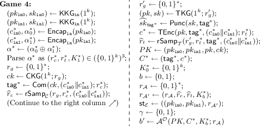
Proof of Theorem  1. Let $\mathcal {A}$ be any PPTA adversary that attacks the $\mathtt {CCA}$ security of the KEM $\varGamma$. Our security proof is via the sequence of games argument. To describe the games, we will need an extractor $\mathcal {E}$ corresponding to some “ciphertext creator” $\mathcal {A}'$ that is guaranteed to exist by the $\mathtt {sPA1}_2$ security of $\varGamma _{\mathtt {in}}$. Specifically, consider the following $\mathcal {A}'$ (that internally runs $\mathcal {A}$) that runs in the experiment $\mathsf {Expt}^{\mathtt {sPA1}}_{\varGamma _{\mathtt {in}}, \mathcal {A}', \mathcal {E}, 2}(k)$, with a corresponding extractor $\mathcal {E}$:

• ${\mathcal {A}'^{\mathcal {E}(\mathsf {st}_{\mathcal {E}}, \cdot )}(pk_1, pk_2; r_{\mathcal {A}'} = (r_{\mathcal {A}}, \widehat{r}_c, \widehat{r}_t, K^*)){\varvec{:}}}$ $\mathcal {A}'$ firstly sets $pk_{\mathtt {in0}}\leftarrow pk_1$ and $pk_{\mathtt {in1}}\leftarrow pk_2$ (which implicitly sets $sk_{\mathtt {in0}}\leftarrow sk_1$ and $sk_{\mathtt {in1}}\leftarrow sk_2$, where $sk_1$ (resp. $sk_2$) is the secret key corresponding to $pk_1$ (resp. $pk_2$)), and runs $(ck, \mathsf {tag}^*) \leftarrow \mathsf {oSamp}_{\mathcal {C}}(1^k; \widehat{r}_c)$ and $(pk, c^*, \widehat{sk}_{\mathsf {tag}^*}) \leftarrow \mathsf {oSamp}_{\mathcal {T}}(\mathsf {tag}^*; \widehat{r}_t)$. Then $\mathcal {A}'$ sets $PK \leftarrow (pk_{\mathtt {in0}}, pk_{\mathtt {in1}}, pk, ck)$ and $C^* \leftarrow (\mathsf {tag}^*, c^*)$, and then runs $\mathcal {A}(PK, C^*, K^*; r_{\mathcal {A}})$.

  When $\mathcal {A}$ submits a decapsulation query C, $\mathcal {A}'$ responds to it as if it runs $\mathsf {AltDecap}(\widehat{SK}_{\mathsf {tag}^*}, C)$, where the oracle calls (to the extractor $\mathcal {E}$) of the form $(1, c_{\mathtt {in0}})$ and $(2, c_{\mathtt {in1}})$ are used as substitutes for $\mathsf {Decap}_{\mathtt {in}}(sk_{\mathtt {in0}}, c_{\mathtt {in0}})$ and $\mathsf {Decap}_{\mathtt {in}}(sk_{\mathtt {in1}}, c_{\mathtt {in1}})$, respectively. More precisely, $\mathcal {A}'$ answers $\mathcal {A}$’s decapsulation query $C = (\mathsf {tag}, c)$ as follows:

  • 1. If $\mathsf {tag}= \mathsf {tag}^*$, then return $\bot$ to $\mathcal {A}$.

  • 2. Run $(c_{\mathtt {in0}}\Vert c_{\mathtt {in1}}) \leftarrow \widehat{\mathsf {TDec}}(\widehat{sk}_{\mathsf {tag}^*}, \mathsf {tag}, c)$, and return $\bot$ to $\mathcal {A}$ if $\widehat{\mathsf {TDec}}$ has returned $\bot$.

  • 3. Submit queries $(1, c_{\mathtt {in0}})$ and $(2, c_{\mathtt {in1}})$ to the extractor $\mathcal {E}(\mathsf {st}_{\mathcal {E}}, \cdot )$ and receive the answers $\alpha _0$ and $\alpha _1$, respectively. (Here, the answers $\alpha _0$ and $\alpha _1$ are expected to be $\alpha _0= \mathsf {Decap}_{\mathtt {in}}(sk_{\mathtt {in0}}, c_{\mathtt {in0}})$ and $\alpha _1= \mathsf {Decap}_{\mathtt {in}}(sk_{\mathtt {in1}}, c_{\mathtt {in1}})$, respectively, and the extractor $\mathcal {E}$ may update its state upon each call).

  • 4. If $\alpha _0= \bot$ or $\alpha _1= \bot$, then return $\bot$ to $\mathcal {A}$.

  • 5. Let $\alpha \leftarrow \alpha _0\oplus \alpha _1$ and parse $\alpha$ as $(r_c, r_t, K) \in (\{0,1\}^k)^3$.

  • 6. If $\mathsf {Com}(ck, (c_{\mathtt {in0}}\Vert c_{\mathtt {in1}}); r_c) = \mathsf {tag}$ and $\mathsf {TEnc}(pk, (c_{\mathtt {in0}}\Vert c_{\mathtt {in1}}); r_t) = c$, then return K, otherwise return $\bot$, to $\mathcal {A}$. When $\mathcal {A}$ terminates, $\mathcal {A}'$ also terminates.

The above completes the description of the algorithm $\mathcal {A}'$. The randomness $r_{\mathcal {A}'}$ consumed by $\mathcal {A}'$ is of the form $(r_{\mathcal {A}}, \widehat{r}_c, \widehat{r}_t, K^*)$, where $r_{\mathcal {A}}$, $\widehat{r}_c$, and $\widehat{r}_t$ are the randomness used by $\mathcal {A}$, $\mathsf {oSamp}_{\mathcal {C}}$, and $\mathsf {oSamp}_{\mathcal {T}}$, respectively, and $K^*$ is a k-bit string. The corresponding extractor $\mathcal {E}$ thus receives $(pk_1, pk_2)$ and $r_{\mathcal {A}'}$ as its initial state $\mathsf {st}_{\mathcal {E}}$. Note that since $\varGamma _{\mathtt {in}}$ is assumed to be $\mathtt {sPA1}_2$ secure and $\mathcal {A}'$ is a PPTA, $\mathsf {Adv}^{\mathtt {sPA1}}_{\varGamma _{\mathtt {in}}, \mathcal {A}', \mathcal {E}, 2}(k)$ is negligible for this extractor $\mathcal {E}$, which will be used later in the proof. (Looking ahead, we will design the sequence of games so that $\mathcal {A}$’s view in the case $\mathcal {A}$ is internally run by $\mathcal {A}'$ and $\mathcal {A}'$ is run in $\mathsf {Expt}^{\mathtt {sPA1}}_{\varGamma _{\mathtt {in}},\mathcal {A}',\mathcal {E},2}(k)$, is identical to $\mathcal {A}$’s view in Game 6).

For convenience, we refer to the procedure of using the extractor $\mathcal {E}$ as substitutes for $\mathsf {Decap}_{\mathtt {in}}(sk_{\mathtt {in0}}, \cdot )$ and $\mathsf {Decap}_{\mathtt {in}}(sk_{\mathtt {in1}}, \cdot )$, as $\mathsf {AltDecap}'_{\mathcal {E}}$. Here, $\mathsf {AltDecap}'_{\mathcal {E}}$ is a stateful procedure that initially takes $\mathsf {tag}^*$, $\widehat{sk}_{\mathsf {tag}^*}$, and an initial state $\mathsf {st}_{\mathcal {E}}$ of $\mathcal {E}$ (i.e. $\mathsf {st}_{\mathcal {E}} = ((pk_{\mathtt {in0}}, pk_{\mathtt {in1}}), r_{\mathcal {A}'})$) as input, and expects to receive a ciphertext $C = (\mathsf {tag}, c)$ as an input. If it receives a ciphertext $C = (\mathsf {tag}, c)$, it calculates the decapsulation result K (or $\bot$) as $\mathcal {A}'$ does for $\mathcal {A}$, using $\widehat{sk}_{\mathsf {tag}^*}$ and the extractor $\mathcal {E}$, where $\mathcal {E}$’s internal state could be updated upon each execution.

Now, using the adversary $\mathcal {A}$ and the extractor $\mathcal {E}$, consider the following sequence of games: (Here, the values with asterisk (*) represent those related to the challenge ciphertext for $\mathcal {A}$).

• Game 1: This is the experiment $\mathsf {Expt}^{\mathtt {CCA}}_{\varGamma , \mathcal {A}}(k)$ itself.

• Game 2: Same as Game 1, except that all decapsulation queries $C = (\mathsf {tag}, c)$ satisfying $\mathsf {tag}= \mathsf {tag}^*$ are answered with $\bot$.

• Game 3: Same as Game 2, except that all decapsulation queries C are answered with $\mathsf {AltDecap}(\widehat{SK}_{\mathsf {tag}^*}, C)$, where $\widehat{SK}_{\mathsf {tag}^*}$ is the alternative secret key corresponding to (PK, SK) and $\mathsf {tag}^*$. Furthermore, we pick a random bit $\gamma \in \{0,1\}$ uniformly at random just before executing $\mathcal {A}$, which will be used to define the events in this game and the subsequent games. ($\gamma$ does not appear in $\mathcal {A}$’s view in this and all subsequent games, and thus does not affect its behavior at all).

• Game 4: In this game, we use $\mathsf {AltDecap}'_{\mathcal {E}}$ (defined as above) as $\mathcal {A}$’s decapsulation oracle, where the initial state of $\mathcal {E}$ (used internally by $\mathsf {AltDecap}'_{\mathcal {E}}$) is prepared using the “inverting algorithms” $\mathsf {rSamp}_{\mathcal {C}}$ of $\mathcal {C}$ and $\mathsf {rSamp}_{\mathcal {T}}$ of $\mathcal {T}$. Moreover, we also change the ordering of the steps so that they do not affect $\mathcal {A}$’s view. More precisely, this game is defined as follows:

  

  where the decapsulation oracle $\mathcal {O}$ that $\mathcal {A}$ has access in Game 4 is $\mathsf {AltDecap}'_{\mathcal {E}}$ (which initially receives $\mathsf {tag}^*, \widehat{sk}_{\mathsf {tag}^*}, \mathsf {st}_{\mathcal {E}} = (pk_{\mathtt {in0}}, pk_{\mathtt {in1}}, r_{\mathcal {A}'})$ as input). Note that the extractor $\mathcal {E}$ used internally by $\mathsf {AltDecap}'_{\mathcal {E}}$ may update its state $\mathsf {st}_{\mathcal {E}}$ upon each execution.

• Game 5: Same as Game 4, except that $r^*_c, r^*_t, K^*_1 \in \{0,1\}^k$ are picked uniformly at random, independently of $\alpha ^* = \alpha _0^* \oplus \alpha _1^*$. That is, the steps “$\alpha ^* \leftarrow \alpha _0^* \oplus \alpha _1^*$; Parse $\alpha ^*$ as $(r^*_c,r^*_t,K^*_1) \in (\{0,1\}^k)^3$” in Game 4 are replaced with the step “$r^*_c, r^*_t, K^*_1 \leftarrow \{0,1\}^k$,” and we do not use $\alpha ^*$ anymore.

• Game 6: Same as Game 5, except that the key/commitment pair $(ck, \mathsf {tag}^*)$ and the key/ciphertext pair $(pk, c^*)$ and a punctured secret key $\widehat{sk}_{\mathsf {tag}^*}$ are sampled obliviously, and correspondingly the randomness $\widehat{r}_c$ and $\widehat{r}_t$ used for oblivious sampling are used in $r_{\mathcal {A}'}$.

  More precisely, the steps “$r_g, r^*_c \leftarrow \{0,1\}^*$; $ck \leftarrow \mathsf {CKG}(1^k; r_g)$; $\mathsf {tag}^* \leftarrow \mathsf {Com}(ck, (c_{\mathtt {in0}}^* \Vert c_{\mathtt {in1}}^*); r^*_c)$; $\widehat{r}_c \leftarrow \mathsf {rSamp}_{\mathcal {C}}(r_g, r^*_c, (c_{\mathtt {in0}}^* \Vert c_{\mathtt {in1}}^*))$” in Game 5 are replaced with the steps “$\widehat{r}_c \leftarrow \{0,1\}^*$; $(ck, \mathsf {tag}^*) \leftarrow \mathsf {oSamp}_{\mathcal {C}}(1^k; \widehat{r}_c)$”. Furthermore, the steps “$r'_g, r^*_t \leftarrow \{0,1\}^k$; $(pk, sk) \leftarrow \mathsf {TKG}(1^k; r'_g)$; $c^* \leftarrow \mathsf {TEnc}(pk, \mathsf {tag}^*, (c_{\mathtt {in0}}^* \Vert c_{\mathtt {in1}}^*); r^*_t)$; $\widehat{r}_t \leftarrow \mathsf {rSamp}_{\mathcal {T}}(r'_g, r^*_t, \mathsf {tag}^*, (c_{\mathtt {in0}}^* \Vert c_{\mathtt {in1}}^*))$” in Game 5 are replaced with the steps “$\widehat{r}_t \leftarrow \{0,1\}^*$; $(pk, \widehat{sk}_{\mathsf {tag}^*}, c^*) \leftarrow \mathsf {oSamp}_{\mathcal {T}}(\mathsf {tag}^*; \widehat{r}_t)$”.

The above completes the description of the games.

For $i\,\in$ [5], let $\mathsf {Succ}_i$ denote the event that $\mathcal {A}$ succeeds in guessing the challenge bit (i.e. $b' = b$ occurs) in Game i. Furthermore, for $i \in \{3,\dots ,6\}$, we define the following bad events in Game i:

• $\mathsf {Bad}_i{\varvec{:}}$ $\mathcal {A}$ submits a decapsulation query $C = (\mathsf {tag}, c)$ satisfying the following conditions simultaneously: (1) $\mathsf {tag}\ne \mathsf {tag}^*$, (2) $\widehat{\mathsf {TDec}}(\widehat{sk}_{\mathsf {tag}^*}, \mathsf {tag}, c) = (c_{\mathtt {in0}}\Vert c_{\mathtt {in1}}) \ne \bot$, and (3) $\mathsf {Decap}_{\mathtt {in}}(sk_{\mathtt {in0}}, c_{\mathtt {in0}}) \ne \mathcal {E}(\mathsf {st}_{\mathcal {E}}, (1, c_{\mathtt {in0}}))$ or $\mathsf {Decap}_{\mathtt {in}}(sk_{\mathtt {in1}}, c_{\mathtt {in1}}) \ne \mathcal {E}(\mathsf {st}_{\mathcal {E}}, (2, c_{\mathtt {in1}}))$.

• $\mathsf {Bad}^{(\sigma )}_i{\varvec{:}}$ (where $\sigma \in \{0,1\}$) $\mathcal {A}$ submits a decapsulation query $C = (\mathsf {tag}, c)$ that satisfies the same conditions as $\mathsf {Bad}_i$, except that the condition (3) is replaced with the condition: $\mathsf {Decap}_{\mathtt {in}}(sk_{\mathtt {in}\sigma }, c_{\mathtt {in}\sigma }) \ne \mathcal {E}(\mathsf {st}_{\mathcal {E}}, (\sigma + 1, c_{\mathtt {in}\sigma }))$.

• $\mathsf {Bad}^*_i{\varvec{:}}$ $\mathcal {A}$ submits a decapsulation query $C = (\mathsf {tag}, c)$ that satisfies the same conditions as $\mathsf {Bad}_i$, except that the condition (3) is replaced with the condition: $\mathsf {Decap}_{\mathtt {in}}(sk_{\mathtt {in}\gamma }, c_{\mathtt {in}\gamma }) \ne \mathcal {E}(\mathsf {st}_{\mathcal {E}}, (\gamma + 1, c_{\mathtt {in}\gamma }))$ (where $\gamma$ is the random bit chosen just before executing $\mathcal {A}$).

Note that for all $i \in \{3,\dots ,6\}$, the events $\mathsf {Bad}^{(0)}_i$, $\mathsf {Bad}^{(1)}_i$, and $\mathsf {Bad}^*_i$ all imply the event $\mathsf {Bad}_i$, and thus we have $\Pr [\mathsf {Bad}^{(0)}_i], \Pr [\mathsf {Bad}^{(1)}_i], \Pr [\mathsf {Bad}^*_i] \le \Pr [\mathsf {Bad}_i]$.

By the definitions of the games and events, we have

$$\begin{aligned} \mathsf {Adv}^{\mathtt {CCA}}_{\varGamma , \mathcal {A}}(k)&= 2 \cdot \Bigl | \Pr [\mathsf {Succ}_1] - \frac{1}{2} \Bigr | \nonumber \\&\le 2 \cdot \Bigl (~\sum _{i \in [4]} \Bigl | \Pr [\mathsf {Succ}_i] - \Pr [\mathsf {Succ}_{i+1}] \Bigr | + \Bigl | \Pr [\mathsf {Succ}_5] - \frac{1}{2} \Bigr |~\Bigr ). \end{aligned}$$

(1)

In the following, we will upperbound each term that appears in the right hand side of the above inequality.

Claim 1

There exists a PPTA $\mathcal {B}_{\mathtt {b}}$ such that $\mathsf {Adv}^{\mathtt {TBind}}_{\mathcal {C},\mathcal {B}_{\mathtt {b}}}(k) \ge |\Pr [\mathsf {Succ}_1] - \Pr [\mathsf {Succ}_2]|$.

Proof of Claim 1. For $i \in \{1,2\}$, let $\mathsf {NoBind}_i$ be the event that in Game i, $\mathcal {A}$ submits at least one decapsulation query $C = (\mathsf {tag}, c)$ satisfying $\mathsf {tag}= \mathsf {tag}^*$ and $\mathsf {Decap}(SK, C) \ne \bot$. Recall that $\mathcal {A}$’s query C must satisfy $C \ne C^* = (\mathsf {tag}^*, c^*)$, and thus $\mathsf {tag}= \mathsf {tag}^*$ implies $c \ne c^*$. The difference between Game 1 and Game 2 is how $\mathcal {A}$’s decapsulation query $C = (\mathsf {tag}, c)$ satisfying $\mathsf {tag}= \mathsf {tag}^*$ is answered. Hence, these games proceed identically unless $\mathsf {NoBind}_1$ or $\mathsf {NoBind}_2$ occurs in the corresponding games, and thus we have

$$\begin{aligned} \Bigl | \Pr [\mathsf {Succ}_1] - \Pr [\mathsf {Succ}_2] \Bigr | \le \Pr [\mathsf {NoBind}_1] = \Pr [\mathsf {NoBind}_2]. \end{aligned}$$

(2)

Thus, it is sufficient to upperbound $\Pr [\mathsf {NoBind}_2]$.

Observe that for a decapsulation query $C = (\mathsf {tag}^*, c)$ satisfying the condition of $\mathsf {NoBind}_2$, it is guaranteed that $\mathsf {TDec}(sk, \mathsf {tag}, c) = (c_{\mathtt {in0}}\Vert c_{\mathtt {in1}}) \ne (c_{\mathtt {in0}}^* \Vert c_{\mathtt {in1}}^*)$. Indeed, if $\mathsf {TDec}(sk, \mathsf {tag}, c) = (c_{\mathtt {in0}}^* \Vert c_{\mathtt {in1}}^*)$ and $\mathsf {Decap}(SK, C) \ne \bot$, then by the validity check of c in $\mathsf {Decap}$, we have $c^* = c$, which is because c must satisfy $\mathsf {TEnc}(pk, \mathsf {tag}^*, (c_{\mathtt {in0}}^* \Vert c_{\mathtt {in1}}^*); r^*_t) = c$ where $r^*_t$ is the $(k+1)$-to-2k-th bits of $\alpha ^* = (\alpha _0^* \oplus \alpha _1^*) = (\mathsf {Decap}_{\mathtt {in}}(sk_{\mathtt {in0}}, c_{\mathtt {in0}}^*) \oplus \mathsf {Decap}_{\mathtt {in}}(sk_{\mathtt {in1}}, c_{\mathtt {in1}}^*))$. However, $\mathsf {TEnc}(pk, \mathsf {tag}^*, (c_{\mathtt {in0}}^* \Vert c_{\mathtt {in1}}^*); r^*_t) = c^*$ also holds due to how $c^*$ is generated, and thus contradicting the condition $c \ne c^*$ implied by $\mathsf {NoBind}_2$.

We use the above fact to show how to construct a PPTA adversary $\mathcal {B}_{\mathtt {b}}$ that attacks the target-binding property of the commitment scheme $\mathcal {C}$ with advantage $\mathsf {Adv}^{\mathtt {TBind}}_{\mathcal {C},\mathcal {B}_{\mathtt {b}}}(k) = \Pr [\mathsf {NoBind}_2]$. The description of $\mathcal {B}_{\mathtt {b}} = (\mathcal {B}_{\mathtt {b}1}, \mathcal {B}_{\mathtt {b}2})$ is as follows:

• $\mathcal {B}_{\mathtt {b}1}(1^k){\varvec{:}}$ $\mathcal {B}_{\mathtt {b}1}$ first runs $(pk_{\mathtt {in0}}, sk_{\mathtt {in0}}) \leftarrow \mathsf {KKG}_{\mathtt {in}}(1^k)$, $(pk_{\mathtt {in1}}, sk_{\mathtt {in1}}) \leftarrow \mathsf {KKG}_{\mathtt {in}}(1^k)$, $(c_{\mathtt {in0}}^*, \alpha _0^*) \leftarrow \mathsf {Encap}_{\mathtt {in}}(pk_{\mathtt {in0}})$, and $(c_{\mathtt {in1}}^*, \alpha _1^*) \leftarrow \mathsf {Encap}_{\mathtt {in}}(pk_{\mathtt {in1}})$. $\mathcal {B}_{\mathtt {b}1}$ then sets $\alpha ^* \leftarrow (\alpha _0^* \oplus \alpha _1^*)$, and parses $\alpha ^*$ as $(r^*_c, r^*_t, \alpha ^*) \in (\{0,1\}^k)^3$. Finally, $\mathcal {B}_{\mathtt {b}1}$ sets $M \leftarrow (c_{\mathtt {in0}}^* \Vert c_{\mathtt {in1}}^*)$, $R \leftarrow r^*_c$, and $\mathsf {st}_{\mathcal {B}} \leftarrow (\mathcal {B}_{\mathtt {b}1}\text {'s entire view})$, and terminates with output $(M, R, \mathsf {st}_{\mathcal {B}})$.

• $\mathcal {B}_{\mathtt {b}2}(\mathsf {st}_{\mathcal {B}}, ck){\varvec{:}}$ $\mathcal {B}_{\mathtt {b}2}$ first runs $(pk, sk) \leftarrow \mathsf {TKG}(1^k)$, and then sets $PK \leftarrow (pk_{\mathtt {in0}}, pk_{\mathtt {in1}}, pk, ck)$ and $SK \leftarrow (sk_{\mathtt {in0}}, sk_{\mathtt {in1}}, sk, PK)$. $\mathcal {B}_{\mathtt {b}2}$ next runs $\mathsf {tag}^* \leftarrow \mathsf {Com}(ck, (c_{\mathtt {in0}}^* \Vert c_{\mathtt {in1}}^*); r^*_c)$ and $c^* \leftarrow \mathsf {TEnc}(pk, \mathsf {tag}^*, (c_{\mathtt {in0}}^* \Vert c_{\mathtt {in1}}^*); r^*_t)$, sets $C^* \leftarrow (\mathsf {tag}^*, c^*)$, and also chooses $K^*_0 \in \{0,1\}^k$ and $b \in \{0,1\}$ uniformly at random. Then, $\mathcal {B}_{\mathtt {b}2}$ runs $\mathcal {A}$, where the decapsulation queries from $\mathcal {A}$ are answered as Game 2 does, which is possible because $\mathcal {B}_{\mathtt {b}2}$ possesses SK.

  When $\mathcal {A}$ terminates, $\mathcal {B}_{\mathtt {b}2}$ checks if $\mathcal {A}$ has made a decapsulation query $C = (\mathsf {tag}, c)$ satisfying the conditions of $\mathsf {NoBind}_2$, namely, $\mathsf {tag}= \mathsf {tag}^*$, $c \ne c^*$, $\mathsf {TDec}(sk, \mathsf {tag}, c) = (c_{\mathtt {in0}}\Vert c_{\mathtt {in1}}) \notin \{(c_{\mathtt {in0}}^* \Vert c_{\mathtt {in1}}^*), \bot \}$, $\mathsf {Decap}_{\mathtt {in}}(sk_{\mathtt {in0}}, c_{\mathtt {in0}}) = \alpha _0\ne \bot$, $\mathsf {Decap}_{\mathtt {in}}(sk_{\mathtt {in1}}, c_{\mathtt {in1}}) = \alpha _1\ne \bot$, $(\alpha _0\oplus \alpha _1) = (r_c \Vert r_t \Vert K) \in \{0,1\}^{3k}$, and $\mathsf {Com}(ck, (c_{\mathtt {in0}}\Vert c_{\mathtt {in1}}); r_c) = \mathsf {tag}^*$, and $\mathsf {TEnc}(pk, \mathsf {tag}, (c_{\mathtt {in0}}\Vert c_{\mathtt {in1}}); r_t) = c$. (Actually, the last condition is redundant for $\mathcal {B}_{\mathtt {b}2}$’s purpose). If such a query is found, then $\mathcal {B}_{\mathtt {b}2}$ terminates with output $M' = (c_{\mathtt {in0}}\Vert c_{\mathtt {in1}})$ and $R' = r_c$. Otherwise, $\mathcal {B}_{\mathtt {b}2}$ gives up and aborts.

The above completes the description of $\mathcal {B}_{\mathtt {b}}$. It is easy to see that $\mathcal {B}_{\mathtt {b}}$ does a perfect simulation of Game 2 for $\mathcal {A}$, and whenever $\mathcal {A}$ makes a query that causes the event $\mathsf {NoBind}_2$, $\mathcal {B}_{\mathtt {b}2}$ can find such a query by using SK and output a pair $(M', R') = ((c_{\mathtt {in0}}\Vert c_{\mathtt {in1}}), r_c)$ satisfying $\mathsf {Com}(ck, M; R) = \mathsf {Com}(ck, M'; R') = \mathsf {tag}^*$ and $M \ne M'$, violating the target-binding property of the commitment scheme $\mathcal {C}$. Therefore, we have $\mathsf {Adv}^{\mathtt {TBind}}_{\mathcal {C}, \mathcal {B}_{\mathtt {b}}}(k) = \Pr [\mathsf {NoBind}_2]$. Then, by Eq. (2), we have $\mathsf {Adv}^{\mathtt {TBind}}_{\mathcal {C}, \mathcal {B}_{\mathtt {b}}}(k) \ge |\Pr [\mathsf {Succ}_1] - \Pr [\mathsf {Succ}_2]|$, as required.    $\square$ (Claim 1)

Claim 2

$\Pr [\mathsf {Succ}_2] = \Pr [\mathsf {Succ}_3]$.

Proof of Claim 2. It is sufficient to show that the behavior of the oracle given to $\mathcal {A}$ in Game 2 and that in Game 3 are identical. Let $C = (\mathsf {tag}, c)$ be a decapsulation query that $\mathcal {A}$ makes. If $\mathsf {tag}= \mathsf {tag}^*$, then the query is answered with $\bot$ in Game 2 by definition, while the oracle $\mathsf {AltDecap}(\widehat{SK}_{\mathsf {tag}^*}, C)$ that is given access to $\mathcal {A}$ in Game 3 also returns $\bot$ by definition. Otherwise (i.e. $\mathsf {tag}\ne \mathsf {tag}^*$), by Lemma 3, the result of $\mathsf {Decap}(SK, C)$ and that of $\mathsf {AltDecap}(\widehat{SK}_{\mathsf {tag}^*}, C)$ always agree. This completes the proof.    $\square$ (Claim 2)

Claim 3

There exist PPTAs $\mathcal {B}_{\mathtt {g}}$ and $\mathcal {B}_{\mathtt {d}}$ such that

$$ \Bigl | \Pr [\mathsf {Succ}_3] - \Pr [\mathsf {Succ}_4] \Bigr | \le 2 \cdot \left( \mathsf {Adv}^{\mathtt {CPA}}_{\varGamma _{\mathtt {in}}, \mathcal {B}_{\mathtt {g}}}(k) + \mathsf {Adv}^{\mathtt {TS}}_{[\mathcal {C},\mathcal {T}],\mathcal {B}_{\mathtt {d}}}(k) + \mathsf {Adv}^{\mathtt {sPA1}}_{\varGamma _{\mathtt {in}}, \mathcal {A}', \mathcal {E}, 2}(k) \right) . $$

We postpone the proof of this claim to the end of the proof of Theorem 1.

Claim 4

There exists a PPTA $\mathcal {B}'_{\mathtt {g}}$ such that $\mathsf {Adv}^{\mathtt {CPA}}_{\varGamma _{\mathtt {in}}, \mathcal {B}'_{\mathtt {g}}}(k) = |\Pr [\mathsf {Succ}_4] - \Pr [\mathsf {Succ}_5]|$.

Proof of Claim 4.  Using $\mathcal {A}$ and $\mathcal {E}$ as building blocks, we show how to construct a PPTA $\mathtt {CPA}$ adversary $\mathcal {B}'_{\mathtt {g}}$ with the claimed advantage. The description of $\mathcal {B}'_{\mathtt {g}}$ is as follows:

• $\mathcal {B}'_{\mathtt {g}}(pk', c'^*, \alpha '^*_\beta ){\varvec{:}}$ (where $\beta \in \{0,1\}$ is $\mathcal {B}'_{\mathtt {g}}$’s challenge bit in its $\mathtt {CPA}$ experiment) $\mathcal {B}'_{\mathtt {g}}$ sets $pk_{\mathtt {in0}}\leftarrow pk'$, $c_{\mathtt {in0}}^* \leftarrow c'^*$, and $\alpha _0^* \leftarrow \alpha '^*_{\beta }$. Next, $\mathcal {B}'_{\mathtt {g}}$ generates $(pk_{\mathtt {in1}}, sk_{\mathtt {in1}}) \leftarrow \mathsf {KKG}_{\mathtt {in}}(1^k)$ and $(c_{\mathtt {in1}}^*, \alpha _1^*) \leftarrow \mathsf {Encap}_{\mathtt {in}}(pk_{\mathtt {in1}})$, sets $\alpha ^* \leftarrow (\alpha _0^* \oplus \alpha _1^*)$, and parses $\alpha ^*$ as $(r^*_c, r^*_t, K^*_1) \in (\{0,1\}^k)^3$. Then, $\mathcal {B}'_{\mathtt {g}}$ picks $r_g, r'_g \leftarrow \{0,1\}^*$ uniformly at random, and runs $ck \leftarrow \mathsf {CKG}(1^k; r_g)$, $\mathsf {tag}^* \leftarrow \mathsf {Com}(ck, (c_{\mathtt {in0}}^* \Vert c_{\mathtt {in1}}^*); r^*_c)$, $\widehat{r}_c \leftarrow \mathsf {rSamp}_{\mathcal {C}}(r_g, r^*_c, (c_{\mathtt {in0}}^* \Vert c_{\mathtt {in1}}^*))$, $(pk, sk) \leftarrow \mathsf {TKG}(1^k; r'_g)$, $\widehat{sk}_{\mathsf {tag}^*} \leftarrow \mathsf {Punc}(sk, \mathsf {tag}^*)$, $c^* \leftarrow \mathsf {TEnc}(pk, \mathsf {tag}^*, (c_{\mathtt {in0}}^* \Vert c_{\mathtt {in1}}^*); r^*_t)$, and $\widehat{r}_t \leftarrow \mathsf {rSamp}_{\mathcal {T}}(r'_g, r^*_t, \mathsf {tag}^*, (c_{\mathtt {in0}}^* \Vert c_{\mathtt {in1}}^*))$. Then $\mathcal {B}'_{\mathtt {g}}$ picks $r_{\mathcal {A}} \in \{0,1\}^*$, $K^*_0 \in \{0,1\}^k$, and $b \in \{0,1\}$ all uniformly at random, and sets $PK \leftarrow (pk_{\mathtt {in0}}, pk_{\mathtt {in1}}, pk, ck)$, $C^* \leftarrow (\mathsf {tag}^*, c^*)$, $r_{\mathcal {A}'} \leftarrow (r_{\mathcal {A}}, \widehat{r}_c, \widehat{r}_t, K^*_b)$, and $\mathsf {st}_{\mathcal {E}} \leftarrow (pk_{\mathtt {in0}}, pk_{\mathtt {in1}}, r_{\mathcal {A}'})$. Finally, $\mathcal {B}'_{\mathtt {g}}$ runs $\mathcal {A}(PK, C^*, K^*_b; r_{\mathcal {A}})$.

  $\mathcal {B}'_{\mathtt {g}}$ answers $\mathcal {A}$’s decapsulation queries as $\mathsf {AltDecap}'_{\mathcal {E}}$ does, where the initial state of $\mathsf {AltDecap}'_{\mathcal {E}}$ is $\mathsf {tag}^*$, $\widehat{sk}_{\mathsf {tag}^*}$, and $\mathsf {st}_{\mathcal {E}}$. (Note that $\mathsf {st}_{\mathcal {E}}$ is used by $\mathcal {E}$, and may be updated upon each call of $\mathsf {AltDecap}'_{\mathcal {E}}$).

  When $\mathcal {A}$ terminates with output $b'$, $\mathcal {B}'_{\mathtt {g}}$ sets $\beta ' \leftarrow (b' \mathop {=}\limits ^{?}b)$, and terminates with output $\beta '$.

The above completes the description of $\mathcal {B}'_{\mathtt {g}}$. $\mathcal {B}'_{\mathtt {g}}$’s $\mathtt {CPA}$ advantage can be calculated as follows:

$$\begin{aligned} \mathsf {Adv}^{\mathtt {CPA}}_{\varGamma _{\mathtt {in}}, \mathcal {B}'_{\mathtt {g}}}(k)&= 2 \cdot \Bigl | \Pr [\beta ' = \beta ] - \frac{1}{2} \Bigr | = \Bigl | \Pr [\beta ' = 1 | \beta = 1] - \Pr [\beta ' = 1| \beta = 0] \Bigr |\\&= \Bigl | \Pr [b' = b | \beta = 1] - \Pr [b' = b| \beta = 0] \Bigr |. \end{aligned}$$

Consider the case when $\beta = 1$. It is easy to see that in this case, $\mathcal {B}'_{\mathtt {g}}$ simulates Game 4 perfectly for $\mathcal {A}$. Specifically, the real session-key $\alpha '^*_{\beta } = \alpha '^*_1$ (corresponding to $c_{\mathtt {in0}}^* = c'^*$) is used as $\alpha _0^*$, and thus $\alpha ^* = (\alpha _0^* \oplus \alpha _1^*) = (r^*_c \Vert r^*_t \Vert K^*_1)$ is generated exactly as that in Game 4. All other values are distributed identically to those in Game 4. Furthermore, $\mathcal {B}'_{\mathtt {g}}$ uses $\mathsf {AltDecap}'_{\mathcal {E}}$ for answering $\mathcal {A}$’s decapsulation queries, where the initial state of $\mathsf {AltDecap}'_{\mathcal {E}}$ (and thus the initial state of $\mathcal {E}$) is appropriately generated as those in Game 4. Under this situation, the probability that $\mathcal {A}$ succeeds in guessing b (i.e. $b' = b$ occurs) is exactly the same as the probability that $\mathcal {A}$ does so in Game 4, i.e. $\Pr [b' = b | \beta = 1] = \Pr [\mathsf {Succ}_4]$.

On the other hand, when $\beta = 0$, then $\mathcal {B}'_{\mathtt {g}}$ simulates Game 5 perfectly for $\mathcal {A}$. Specifically, in this case, a uniformly random value $\alpha '^*_{\beta } = \alpha '^*_0$ is used as $\alpha _0^*$. Therefore, $\alpha ^* = (\alpha _0^* \oplus \alpha _1^*)$ is also a uniformly random 3k-bit string, and thus each of $r^*_c$, $r^*_t$, and $K^*_1$ is a uniformly random k-bit string, which is exactly how these values are chosen in Game 5. Since this is the only change from the case of $\beta = 1$, with a similar argument to the above, we have $\Pr [b' = b | \beta = 0] = \Pr [\mathsf {Succ}_5]$.

In summary, we have $\mathsf {Adv}^{\mathtt {CPA}}_{\varGamma _{\mathtt {in}}, \mathcal {B}'_{\mathtt {g}}}(k) = |\Pr [\mathsf {Succ}_4] - \Pr [\mathsf {Succ}_5]|$, as required.   $\square$ (Claim 4)

Claim 5

$\Pr [\mathsf {Succ}_5] = 1/2$.

Proof of Claim 5.  This is obvious because in Game 5, the real session-key $K^*_1$ is made independent of the challenge ciphertext $C^*$. Since both $K^*_1$ and $K^*_0$ are now uniformly random, the view of $\mathcal {A}$ does not contain any information on b. This means that the probability that $\mathcal {A}$ succeeds in guessing the challenge bit is exactly $1{\slash }2$.    $\square$ (Claim 5)

Claims 1, 2, 3, 4 and 5 and Eq. (1) guarantee that there exist PPTAs $\mathcal {B}_{\mathtt {b}}$, $\mathcal {B}_{\mathtt {g}}$, $\mathcal {B}_{\mathtt {d}}$, and $\mathcal {B}'_{\mathtt {g}}$ such that

$$\begin{aligned}&\mathsf {Adv}^{\mathtt {CCA}}_{\varGamma , \mathcal {A}}(k) \le 2 \cdot \mathsf {Adv}^{\mathtt {TBind}}_{\mathcal {C}, \mathcal {B}_{\mathtt {b}}}(k) + 4 \cdot \mathsf {Adv}^{\mathtt {CPA}}_{\varGamma _{\mathtt {in}}, \mathcal {B}_{\mathtt {g}}}(k) + 4 \cdot \mathsf {Adv}^{\mathtt {TS}}_{[\mathcal {C},\mathcal {T}], \mathcal {B}_{\mathtt {d}}}(k)\\&\qquad \qquad \qquad \qquad \qquad \qquad \quad \;\;\, + \, 4 \cdot \mathsf {Adv}^{\mathtt {sPA1}}_{\varGamma _{\mathtt {in}}, \mathcal {A}', \mathcal {E}, 2}(k) + 2 \cdot \mathsf {Adv}^{\mathtt {CPA}}_{\varGamma _{\mathtt {in}}, \mathcal {B}'_{\mathtt {g}}}(k), \end{aligned}$$

which, due to our assumptions on the building blocks and Lemma 2, implies that $\mathsf {Adv}^{\mathtt {CCA}}_{\varGamma ,\mathcal {A}}(k)$ is negligible. Recall that the choice of the PPTA $\mathtt {CCA}$ adversary $\mathcal {A}$ was arbitrarily, and thus for any PPTA $\mathtt {CCA}$ adversary $\mathcal {A}$ we can show a negligible upperbound for $\mathsf {Adv}^{\mathtt {CCA}}_{\varGamma , \mathcal {A}}(k)$ as above.

In order to finish the proof of Theorem 1, it remains to prove Claim 3.

Proof of Claim 3.  Note that the difference between Game 3 and Game 4 is how a query $C = (\mathsf {tag}, c)$ satisfying the conditions of $\mathsf {Bad}_3$ (or $\mathsf {Bad}_4$) is answered, and Game 3 and Game 4 proceed identically unless $\mathsf {Bad}_3$ or $\mathsf {Bad}_4$ occurs in the corresponding games. This means that we have

$$\begin{aligned} \Bigl | \Pr [\mathsf {Succ}_3] - \Pr [\mathsf {Succ}_4] \Bigr | \le \Pr [\mathsf {Bad}_3] = \Pr [\mathsf {Bad}_4]. \end{aligned}$$

(3)

We claim the following:

Subclaim 1

$\Pr [\mathsf {Bad}_4] \le 2 \cdot \Pr [\mathsf {Bad}^*_4]$.

Proof of Subclaim 1.  The argument here is essentially the same as the one used in the proof of Claim 4.13 in [17].

Note that the event $\mathsf {Bad}_4$, $\mathsf {Bad}^{(0)}_4$, $\mathsf {Bad}^{(1)}_4$, and $\mathsf {Bad}^*_4$ are triggered once $\mathcal {A}$ makes a query $C = (\mathsf {tag}, c)$ satisfying the conditions that cause these events. Moreover, by definition, if any of the latter three events occurs, then $\mathsf {Bad}_4$ occurs. Furthermore, the bit $\gamma$ is information-theoretically hidden from $\mathcal {A}$’s view in Game 4. This means that the probability of $\mathsf {Bad}^*_4$ occurring is identical to the probability of the event (in Game 4) that is triggered when (1) $\mathcal {A}$ first makes a query satisfying the conditions of $\mathsf {Bad}_4$, (2) $\gamma$ is picked “on-the-fly” at this point, and then (3) $\mathsf {Decap}_{\mathtt {in}}(sk_{\mathtt {in}\gamma }, c_{\mathtt {in}\gamma }) \ne \mathcal {E}(\mathsf {st}_{\mathcal {E}}, (\gamma + 1, c_{\mathtt {in}\gamma }))$ holds. The probability of this event occurring is $\Pr _{\gamma \leftarrow \{0,1\}}[\mathsf {Bad}_4 \wedge \mathsf {Bad}^{(\gamma )}_4] = \Pr _{\gamma \leftarrow \{0,1\}}[\mathsf {Bad}^{(\gamma )}_4]$ (where the probability is also over Game 4 except the choice of $\gamma$). This can be further estimated as follows:

$$\begin{aligned} \Pr _{\gamma \leftarrow \{0,1\}}[\mathsf {Bad}^{(\gamma )}_4]&= \frac{1}{2} \left( \Pr [\mathsf {Bad}^{(0)}_4] + \Pr [\mathsf {Bad}^{(1)}_4] \right) \\&\ge \frac{1}{2} \Pr [\mathsf {Bad}^{(0)}_4 \vee \mathsf {Bad}^{(1)}_4] = \frac{1}{2} \Pr [\mathsf {Bad}_4], \end{aligned}$$

where we used $\Pr [\mathsf {Bad}^{(0)}_4 \vee \mathsf {Bad}^{(1)}_4] = \Pr [\mathsf {Bad}_4]$, which is by definition.

In summary, we have $\Pr [\mathsf {Bad}^*_4] \ge \frac{1}{2} \Pr [\mathsf {Bad}_4]$, as required.    $\square$ (Subclaim 1)

Using Subclaim 1, we can further estimate $\Pr [\mathsf {Bad}_4]$ as follows:

$$\begin{aligned} \Pr [\mathsf {Bad}_4]&\le 2 \cdot \Pr [\mathsf {Bad}^*_4] \nonumber \\&\le 2 \cdot \Bigl ( \Bigl | \Pr [\mathsf {Bad}^*_4] - \Pr [\mathsf {Bad}^*_5] \Bigr | + \Pr [\mathsf {Bad}^*_5] \Bigr ) \nonumber \\&\le 2 \cdot \Bigl ( \Bigl | \Pr [\mathsf {Bad}^*_4] - \Pr [\mathsf {Bad}^*_5] \Bigr | + \Pr [\mathsf {Bad}_5] \Bigr ) \nonumber \\&\le 2 \cdot \Bigl ( \Bigl | \Pr [\mathsf {Bad}^*_4] - \Pr [\mathsf {Bad}^*_5] \Bigr | + \Bigl | \Pr [\mathsf {Bad}_5] - \Pr [\mathsf {Bad}_6] \Bigr | + \Pr [\mathsf {Bad}_6] \Bigr ), \end{aligned}$$

(4)

where we used $\Pr [\mathsf {Bad}^*_5] \le \Pr [\mathsf {Bad}_5]$ in the third inequality, which is again by definition. It remains to upperbound the right hand side of the above inequality.

Subclaim 2

There exists a PPTA $\mathcal {B}_{\mathtt {g}}$ such that $\mathsf {Adv}^{\mathtt {CPA}}_{\varGamma _{\mathtt {in}}, \mathcal {B}_{\mathtt {g}}}(k) = |\Pr [\mathsf {Bad}^*_4] - \Pr [\mathsf {Bad}^*_5]|$.

Proof of Subclaim 2.  Using $\mathcal {A}$ and $\mathcal {E}$ as building blocks, we show how to construct a PPTA $\mathtt {CPA}$ adversary $\mathcal {B}_{\mathtt {g}}$ with the claimed advantage. The description of $\mathcal {B}_{\mathtt {g}}$ is as follows:

• $\mathcal {B}_{\mathtt {g}}(pk', c'^*, \alpha '^*_\beta ){\varvec{:}}$ (where $\beta \in \{0,1\}$ is $\mathcal {B}_{\mathtt {g}}$’s challenge bit in its $\mathtt {CPA}$ experiment) $\mathcal {B}_{\mathtt {g}}$ picks $\gamma \in \{0,1\}$ uniformly at random, then sets $pk_{\mathtt {in}(1-\gamma )} \leftarrow pk'$, $c_{\mathtt {in}(1-\gamma )}^* \leftarrow c'^*$, and $\alpha _{1-\gamma }^* \leftarrow \alpha '^*_{\beta }$. Next, $\mathcal {B}_{\mathtt {g}}$ generates $(pk_{\mathtt {in}\gamma }, sk_{\mathtt {in}\gamma }) \leftarrow \mathsf {KKG}_{\mathtt {in}}(1^k)$ and $(c^*_{\mathtt {in}\gamma }, \alpha ^*_{\gamma }) \leftarrow \mathsf {Encap}_{\mathtt {in}}(pk_{\mathtt {in}\gamma })$, sets $\alpha ^* \leftarrow (\alpha _0^* \oplus \alpha _1^*)$, and parses $\alpha ^*$ as $(r^*_c, r^*_t, K^*_1) \in (\{0,1\}^k)^3$. Then, $\mathcal {B}_{\mathtt {g}}$ prepares $K^*_1, K^*_0 \in \{0,1\}^k$, $b \in \{0,1\}$, $PK = (pk_{\mathtt {in0}}, pk_{\mathtt {in1}}, pk, c)$, $C^* = (\mathsf {tag}^*, c^*)$, $\widehat{sk}_{\mathsf {tag}^*}$, and $\mathsf {st}_{\mathcal {E}} = (pk_{\mathtt {in0}}, pk_{\mathtt {in1}}, r_{\mathcal {A}'} = (r_{\mathcal {A}}, \widehat{r}_c, \widehat{r}_t, K^*_b))$, exactly as $\mathcal {B}'_{\mathtt {g}}$ in the proof of Claim 4 does. Finally, $\mathcal {B}_{\mathtt {g}}$ runs $\mathcal {A}(PK, C^*, K^*_b; r_{\mathcal {A}})$ until it terminates, where $\mathcal {B}_{\mathtt {g}}$ answers $\mathcal {A}$’s queries in exactly the same way as $\mathcal {B}'_{\mathtt {g}}$ does.

  When $\mathcal {A}$ terminates, $\mathcal {B}_{\mathtt {g}}$ checks whether $\mathcal {A}$ has submitted a decapsulation query $C = (\mathsf {tag}, c)$ that satisfies the conditions of $\mathsf {Bad}^*_4$ (i.e. (1) $\mathsf {tag}\ne \mathsf {tag}^*$, (2) $\widehat{\mathsf {TDec}}(\widehat{sk}_{\mathsf {tag}^*}, \mathsf {tag}, c) = (c_{\mathtt {in0}}\Vert c_{\mathtt {in1}}) \ne \bot$, and (3) $\mathsf {Decap}_{\mathtt {in}}(sk_{\mathtt {in}\gamma }, c_{\mathtt {in}\gamma }) \ne \mathcal {E}(\mathsf {st}_{\mathcal {E}}, c_{\mathtt {in}\gamma })$ hold), which can be checked by using $sk_{\mathtt {in}\gamma }$. If such a query is found, the $\mathcal {B}_{\mathtt {g}}$ sets $\beta ' \leftarrow 1$, otherwise sets $\beta ' \leftarrow 0$, and terminates with output $\beta '$.

The above completes the description of $\mathcal {B}_{\mathtt {g}}$. Let $\mathsf {Bad}^*_{\mathcal {B}}$ be the event that $\mathcal {A}$ submits a decapsulation query that satisfies the conditions (1), (2), and (3) of $\mathsf {Bad}^*_4$, in the experiment simulated by $\mathcal {B}_{\mathtt {g}}$. Note that $\mathcal {B}_{\mathtt {g}}$ outputs $\beta ' = 1$ only when $\mathsf {Bad}^*_{\mathcal {B}}$ occurs. Therefore, $\mathcal {B}_{\mathtt {g}}$’s $\mathtt {CPA}$ advantage can be calculated as follows:

$$\begin{aligned} \mathsf {Adv}^{\mathtt {CPA}}_{\varGamma _{\mathtt {in}}, \mathcal {B}_{\mathtt {g}}}(k)&= 2 \cdot \Bigl | \Pr [\beta ' = \beta ] - \frac{1}{2} \Bigr | = \Bigl | \Pr [\beta ' = 1 | \beta = 1] - \Pr [\beta ' = 1| \beta = 0] \Bigr |\\&= \Bigl | \Pr [\mathsf {Bad}^*_{\mathcal {B}} | \beta = 1] - \Pr [\mathsf {Bad}^*_{\mathcal {B}}| \beta = 0] \Bigr |. \end{aligned}$$

With essentially the same arguments as in the proof of Claim 4, we can see that $\mathcal {B}_{\mathtt {g}}$ does a perfect simulation of Game 4 for $\mathcal {A}$ if $\beta = 1$, and does a perfect simulation of Game 5 for $\mathcal {A}$ if $\beta = 0$. In particular, the only difference from the proof of Claim 4 is in which of the positions $(pk_{\mathtt {in0}}, c_{\mathtt {in0}}^*, \alpha _0^*)$ or $(pk_{\mathtt {in1}}, c_{\mathtt {in1}}^*, \alpha _1^*)$ $\mathcal {B}_{\mathtt {g}}$ embeds $\mathcal {B}_{\mathtt {g}}$’s instance of the $\mathtt {CPA}$ experiment. In the proof of Claim 4, the reduction algorithm $\mathcal {B}'_{\mathtt {g}}$ embeds its challenge into $(pk_{\mathtt {in0}}, c_{\mathtt {in0}}^*, \alpha _0^*)$, while in the current proof, the reduction algorithm $\mathcal {B}_{\mathtt {g}}$ embeds its challenge into $(pk_{\mathtt {in}(1-\gamma )}, c^*_{\mathtt {in}(1-\gamma )}, \alpha ^*_{1-\gamma })$ for a random $\gamma \in \{0,1\}$. It is easy to see that even after this change, if $\beta = 1$, then the view of $\mathcal {A}$ is identical to that in Game 4, and if $\beta = 0$, then the view of $\mathcal {A}$ is identical to that in Game 5.

Under the situation, the probability that $\mathsf {Bad}^*_{\mathcal {B}}$ occurs in the experiment simulated by $\mathcal {B}_{\mathtt {g}}$ in case $\beta = 1$ (resp. $\beta = 0$) is identical to the probability that $\mathsf {Bad}^*_4$ (resp. $\mathsf {Bad}^*_5$) occurs in Game 4 (resp. Game 5), namely, we have $\Pr [\mathsf {Bad}^*_{\mathcal {B}} | \beta = 1] = \Pr [\mathsf {Bad}^*_4]$ and $\Pr [\mathsf {Bad}^*_{\mathcal {B}} | \beta = 0] = \Pr [\mathsf {Bad}^*_5]$.

In summary, we have $\mathsf {Adv}^{\mathtt {CPA}}_{\varGamma _{\mathtt {in}}, \mathcal {B}_{\mathtt {g}}}(k) = |\Pr [\mathsf {Bad}^*_4] - \Pr [\mathsf {Bad}^*_5]|$, as required.    $\square$ (Subclaim 2)

Subclaim 3

There exists a PPTA $\mathcal {B}_{\mathtt {d}}$ such that $\mathsf {Adv}^{\mathtt {TS}}_{[\mathcal {C},\mathcal {T}], \mathcal {B}_{\mathtt {d}}}(k) = |\Pr [\mathsf {Bad}_5] - \Pr [\mathsf {Bad}_6]|$.

Proof of Subclaim 3.  Using $\mathcal {A}$ and $\mathcal {E}$ as building blocks, we show how to construct a PPTA $\mathcal {B}$ that has the claimed advantage in distinguishing the distributions considered in Lemma 2. The description of $\mathcal {B}_{\mathtt {d}} = (\mathcal {B}_{\mathtt {d}1}, \mathcal {B}_{\mathtt {d}2})$ as follows:

• $\mathcal {B}_{\mathtt {d}1}(1^k){\varvec{:}}$ $\mathcal {B}_{\mathtt {d}1}$ runs $(pk_{\mathtt {in0}}, sk_{\mathtt {in0}}) \leftarrow \mathsf {KKG}_{\mathtt {in}}(1^k)$, $(pk_{\mathtt {in1}}, sk_{\mathtt {in1}}) \leftarrow \mathsf {KKG}_{\mathtt {in}}(1^k)$, $(c_{\mathtt {in0}}^*, \alpha _0^*) \leftarrow \mathsf {Encap}_{\mathtt {in}}(pk_{\mathtt {in0}})$, $(c_{\mathtt {in1}}^*, \alpha _1^*) \leftarrow \mathsf {Encap}_{\mathtt {in}}(pk_{\mathtt {in1}})$. Then $\mathcal {B}_{\mathtt {d}1}$ sets $M \leftarrow (c_{\mathtt {in0}}^* \Vert c_{\mathtt {in1}}^*)$ and $\mathsf {st}_{\mathcal {B}} \leftarrow (\mathcal {B}_{\mathtt {d}1}\text {'s entire view})$, and terminates with output $(M, \mathsf {st}_{\mathcal {B}})$.

• $\mathcal {B}_{\mathtt {d}2}(\mathsf {st}_{\mathcal {B}}, ck, \mathsf {tag}^*, pk, c^*, \widehat{sk}_{\mathsf {tag}^*}, \widehat{r}_c, \widehat{r}_t){\varvec{:}}$ $\mathcal {B}_{\mathtt {d}2}$ sets $PK \leftarrow (pk_{\mathtt {in0}}, pk_{\mathtt {in1}}, pk, ck)$ and $C^* \leftarrow (\mathsf {tag}^*, c^*)$, picks $K^* \in \{0,1\}^*$ and $r_{\mathcal {A}} \in \{0,1\}^*$ uniformly at random, and then sets $r_{\mathcal {A}'} \leftarrow (r_{\mathcal {A}}, \widehat{r}_c, \widehat{r}_t, K^*)$ and $\mathsf {st}_{\mathcal {E}} \leftarrow (pk_{\mathtt {in0}}, pk_{\mathtt {in1}}, r_{\mathcal {A}'})$. (Recall that $K^*_0$ and $K^*_1$ in Games 5 and 6 are distributed identically, and thus it is sufficient to choose just a single value $K^*$ and pretend as if $K^*$ is $K^*_b$). Then $\mathcal {B}_{\mathtt {d}2}$ runs $\mathcal {A}(PK, C^*, K^*; r_{\mathcal {A}})$.

  $\mathcal {B}_{\mathtt {d}2}$ answers $\mathcal {A}$’s queries as Game 5 does, which is possible because $\mathcal {B}_{\mathtt {d}2}$ possesses $\widehat{sk}_{\mathsf {tag}^*}$ and $\mathsf {st}_{\mathcal {E}}$, and thus $\mathcal {B}_{\mathtt {d}2}$ can run $\mathsf {AltDecap}'_{\mathcal {E}}$ (which internally runs the extractor $\mathcal {E}(\mathsf {st}_{\mathcal {E}}, \cdot )$).

  When $\mathcal {A}$ terminates, $\mathcal {B}_{\mathtt {d}2}$ checks whether $\mathcal {A}$ has submitted a query that satisfies the conditions of $\mathsf {Bad}_5$, which can be checked by using $sk_{\mathtt {in0}}$ and $sk_{\mathtt {in1}}$ that $\mathcal {B}_{\mathtt {d}2}$ possesses. If such a query is found, then $\mathcal {B}_{\mathtt {d}2}$ outputs 1, otherwise outputs 0, and terminates.

The above completes the description of $\mathcal {B}_{\mathtt {d}}$. Let $\mathsf {Bad}_{\mathcal {B}}$ be the event that $\mathcal {A}$ submits a decapsulation query $C = (\mathsf {tag}, c)$ that satisfies the conditions of $\mathsf {Bad}_5$ in the experiment simulated by $\mathcal {B}_{\mathtt {d}}$ (i.e. the query satisfying (1) $\mathsf {tag}\ne \mathsf {tag}^*$, (2) $\widehat{\mathsf {TDec}}(\widehat{sk}_{\mathsf {tag}^*}, \mathsf {tag}, c) = (c_{\mathtt {in0}}\Vert c_{\mathtt {in1}}) \ne \bot$, and (3) $\mathsf {Decap}_{\mathtt {in}}(sk_{\mathtt {in0}}, c_{\mathtt {in0}}) \ne \mathcal {E}(\mathsf {st}_{\mathcal {E}}, c_{\mathtt {in0}})$ or $\mathsf {Decap}_{\mathtt {in}}(sk_{\mathtt {in1}}, c_{\mathtt {in1}}) \ne \mathcal {E}(\mathsf {st}_{\mathcal {E}}, c_{\mathtt {in1}})$). Note that $\mathcal {B}_{\mathtt {d}}$ submits 1 only when $\mathsf {Bad}_{\mathcal {B}}$ occurs. Therefore, $\mathcal {B}_{\mathtt {d}}$’s advantage $\mathsf {Adv}^{\mathtt {TS}}_{[\mathcal {C},\mathcal {T}], \mathcal {B}_{\mathtt {d}}}(k)$ can be calculated as follows:

$$\begin{aligned} \mathsf {Adv}^{\mathtt {TS}}_{[\mathcal {C},\mathcal {T}], \mathcal {B}_{\mathtt {d}}}(k)&= \Bigl | \Pr [\mathsf {Expt}^{\mathtt {TS}{} \texttt {-}\mathtt {Real}}_{[\mathcal {C},\mathcal {T}], \mathcal {B}_{\mathtt {d}}}(k) = 1] - \Pr [\mathsf {Expt}^{\mathtt {TS}{} \texttt {-}\mathtt {Sim}}_{[\mathcal {C},\mathcal {T}], \mathcal {B}_{\mathtt {d}}}(k) = 1] \Bigr |\\&= \Bigl | \Pr [\mathsf {Expt}^{\mathtt {TS}{} \texttt {-}\mathtt {Real}}_{[\mathcal {C},\mathcal {T}],\mathcal {B}_{\mathtt {d}}} : \mathsf {Bad}_{\mathcal {B}}] - \Pr [\mathsf {Expt}^{\mathtt {TS}{} \texttt {-}\mathtt {Sim}}_{[\mathcal {C},\mathcal {T}],\mathcal {B}_{\mathtt {d}}}(k): \mathsf {Bad}_{\mathcal {B}}] \Bigr |. \end{aligned}$$

Consider the case when $\mathcal {B}_{\mathtt {d}}$ is run in the “real” experiment $\mathsf {Expt}^{\mathtt {TS}{} \texttt {-}\mathtt {Real}}_{[\mathcal {C},\mathcal {T}], \mathcal {B}_{\mathtt {d}}}(k)$. It is easy to see that in this case, $\mathcal {B}_{\mathtt {d}}$ simulates Game 5 perfectly for $\mathcal {A}$. Specifically, ck, pk, $\mathsf {tag}^*$, $c^*$, and $\widehat{sk}_{\mathsf {tag}^*}$ are generated from $\mathsf {CKG}$, $\mathsf {TKG}$, $\mathsf {Com}$, $\mathsf {TEnc}$, and $\mathsf {Punc}$, respectively, in such a way that $\mathsf {tag}^*$ is a commitment of $(c_{\mathtt {in0}}^* \Vert c_{\mathtt {in1}}^*)$ and $c^*$ is an encryption of $(c_{\mathtt {in0}}^* \Vert c_{\mathtt {in1}}^*)$ under the tag $\mathsf {tag}^*$. Furthermore, $\widehat{r}_c$ and $\widehat{r}_t$ are generated from $\mathsf {rSamp}_{\mathcal {C}}$ and $\mathsf {rSamp}_{\mathcal {T}}$, respectively, which is how they are generated in Game 5. Under the situation, the probability that $\mathcal {A}$ submits a decapsulation query that causes the event $\mathsf {Bad}_{\mathcal {B}}$ is exactly the same as the probability that $\mathcal {A}$ does so in Game 5. That is, we have $\Pr [\mathsf {Expt}^{\mathtt {TS}{} \texttt {-}\mathtt {Real}}_{[\mathcal {C},\mathcal {T}], \mathcal {B}_{\mathtt {d}}}(k) : \mathsf {Bad}_{\mathcal {B}}] = \Pr [\mathsf {Bad}_5]$.

On the other hand, consider the case when $\mathcal {B}_{\mathtt {d}}$ is run in the “simulated” experiment $\mathsf {Expt}^{\mathtt {TS}{} \texttt {-}\mathtt {Sim}}_{[\mathcal {C}, \mathcal {T}], \mathcal {B}_{\mathtt {d}}}(k)$. In this case, $\mathcal {B}_{\mathtt {d}}$ simulates Game 6 perfectly for $\mathcal {A}$. Specifically, $(ck, \mathsf {tag}^*)$ and $(pk, c^*, \widehat{sk}_{\mathsf {tag}^*})$ are generated by $\mathsf {oSamp}_{\mathcal {C}}(1^k; \widehat{r}_c)$ and $\mathsf {oSamp}_{\mathcal {T}}(\mathsf {tag}^*; \widehat{r}_t)$ with uniformly chosen randomness $\widehat{r}_c$ and $\widehat{r}_t$, respectively, and this is exactly how these values are generated in Game 6. Since this is the only change from the above case, with a similar argument we have $\Pr [\mathsf {Expt}^{\mathtt {TS}{} \texttt {-}\mathtt {Sim}}_{[\mathcal {C},\mathcal {T}], \mathcal {B}_{\mathtt {d}}}(k) : \mathsf {Bad}_{\mathcal {B}}] = \Pr [\mathsf {Bad}_6]$.

In summary, we have $\mathsf {Adv}^{\mathtt {TS}}_{[\mathcal {C},\mathcal {T}], \mathcal {B}_{\mathtt {d}}}(k) = |\Pr [\mathsf {Bad}_5] - \Pr [\mathsf {Bad}_6]|$, as required.    $\square$ (Subclaim 3)

Subclaim 4

$\mathsf {Adv}^{\mathtt {sPA1}}_{\varGamma _{\mathtt {in}}, \mathcal {A}', \mathcal {E}, 2}(k) = \Pr [\mathsf {Bad}_6]$.

Proof of Subclaim 4.  Note that the view of $\mathcal {A}$ in Game 6 is exactly the same as the view of $\mathcal {A}$ when it is internally run by $\mathcal {A}'$ in the situation where $\mathcal {A}'$ is run in the experiment $\mathsf {Expt}^{\mathtt {sPA1}}_{\varGamma _{\mathtt {in}}, \mathcal {A}', \mathcal {E}, 2}(k)$ with the extractor $\mathcal {E}$. Therefore, the probability that $\mathcal {A}$ submits a query that causes the event $\mathsf {Bad}_6$ in Game 6, is exactly the same as the probability that $\mathcal {A}'$ submits a query to $\mathcal {E}$ that makes the experiment $\mathsf {Expt}^{\mathtt {sPA1}}_{\varGamma _{\mathtt {in}}, \mathcal {A}', \mathcal {E}, 2}(k)$ outputs 1 (i.e. $\mathcal {A}'$ submits a query of the form $(j+1, c_{\mathtt {in}j})$ such that $\mathsf {Decap}_{\mathtt {in}}(sk_{\mathtt {in}j}, c_{\mathtt {in}j}) \ne \mathcal {E}(\mathsf {st}_{\mathcal {E}}, (j +1, c_{\mathtt {in}j}))$ for some $j \in \{0,1\}$).    $\square$ (Subclaim 4)

Equations (3) and (4), and Subclaims 2, 3 and 4 imply Claim 3.    $\square$ (Claim 3)

This concludes the proof of Theorem 1.    $\square$ (Theorem 1)

4.2 Second Construction

Let $\varGamma _{\mathtt {in}}= (\mathsf {KKG}_{\mathtt {in}}, \mathsf {Encap}_{\mathtt {in}}, \mathsf {Decap}_{\mathtt {in}})$ be a KEM whose ciphertext length is $n = n(k)$ and whose session-key space is $\{0,1\}^{3k}$ for k-bit security. Let $\mathcal {T}= (\mathsf {TKG}, \mathsf {TEnc}, \mathsf {TDec}, \mathsf {Punc}, \widehat{\mathsf {TDec}})$ be a PTBE scheme and $\mathcal {C}= (\mathsf {CKG}, \mathsf {Com})$ be a commitment scheme. We require the plaintext space of $\mathsf {TEnc}$ and the message space of $\mathsf {Com}$ to be $\{0,1\}^{n}$, and the randomness space of $\mathsf {TEnc}$ and that of $\mathsf {Com}$ to be $\{0,1\}^k$ for k-bit security. Then, our second proposed KEM $\overline{\varGamma }= (\overline{\mathsf {KKG}}, \overline{\mathsf {Encap}}, \overline{\mathsf {Decap}})$ is constructed as in Fig. 4.

Fig. 4.

The second proposed construction: the KEM $\overline{\varGamma }$ based on a KEM $\varGamma _{\mathtt {in}}$, a commitment scheme $\mathcal {C}$, and a PTBE scheme $\mathcal {T}$.

The security of $\overline{\varGamma }$ is guaranteed by the following theorem.

Theorem 2

Assume that the KEM $\varGamma _{\mathtt {in}}$ is $1\texttt {-}\mathtt {CCA}$ secure and $\mathtt {sPA1}_1$ secure, the commitment scheme $\mathcal {C}$ is target-binding and trapdoor simulatable, and the PTBE scheme $\mathcal {T}$ is trapdoor simulatable. Then, the KEM $\overline{\varGamma }$ constructed as in Fig. 4 is $\mathtt {CCA}$ secure.

The proof of this theorem proceeds very similarly to the proof of Theorem 1, and thus we only explain the difference here, and will give the formal proof in the full version.

Recall that in the proof of Theorem 1, the “bad” queries (for which the extractor fails to extract correct decapsulation results) are dealt with due to the property of “multiple encryption” of two instances of the KEM $\varGamma _{\mathtt {in}}$ with public keys $(pk_{\mathtt {in0}}, pk_{\mathtt {in1}})$. In particular, the reduction algorithm in the proof of Subclaim 2 that attacks the $\mathtt {CPA}$ security of the underlying KEM $\varGamma _{\mathtt {in}}$, uses one of secret keys $sk_{\mathtt {in}\gamma }$ (corresponding to $pk_{\mathtt {in}\gamma }$) to detect whether the bad event occurs, while embedding its $\mathtt {CPA}$ instance regarding $\varGamma _{\mathtt {in}}$ into the other position, i.e. into $(pk_{\mathtt {in}(1 -\gamma )}, c_{\mathtt {in}(1-\gamma )})$. This strategy works thanks to the argument regarding the probabilities given in the proof of Subclaim 1 (which is in turn based on the proof of [17, Claim 4.13]). However, for this argument to work, it seems to us that we inherently have to rely on the $\mathtt {sPA1}_2$ security of $\varGamma _{\mathtt {in}}$, in order for the reduction algorithms (especially, the reduction algorithms attacking the $\mathtt {CPA}$ of $\varGamma _{\mathtt {in}}$) to simulate the decapsulation oracle for an adversary $\mathcal {A}$.

The simple idea employed in our second construction is to change the mechanism of detecting the bad queries by relying on the $1\texttt {-}\mathtt {CCA}$ security of $\varGamma _{\mathtt {in}}$, so that a reduction algorithm can check (by its access to the decapsulation oracle) whether $\mathcal {A}$ has submitted a bad decapsulation query. This allows us to use $\varGamma _{\mathtt {in}}$ only in the “single” key setting, leading to only requiring it to be $\mathtt {sPA1}_1$ secure. By employing this idea, a security analysis similar to the recent constructions [31, 37, 40, 44] works, and for the other parts of the security proof (other than the analysis regarding dealing with the bad decapsulation queries) are essentially the same as those in the proof of Theorem 1. For more details, see the full version.

On the Merits of the Second Construction. Since we need to use a KEM which simultaneously satisfies $1\texttt {-}\mathtt {CCA}$ and $\mathtt {sPA1}_1$ security for our second construction, a natural question would be whether we can construct such a scheme. We note that we can achieve such a KEM from a $\mathtt {CPA}$ secure PKE (or a KEM) which is also $\mathtt {sPA1}_{2k}$ secure. Specifically, Dodis and Fiore [21, Appendix C] showed how to construct a $1\texttt {-}\mathtt {CCA}$ secure PKE scheme from the combination of a $\mathtt {CPA}$ secure PKE scheme and a one-time secure signature scheme (in which 2k independently generated public keys are arranged as in the “DDN-lite” construction, but a message is encoded and encrypted in a k-out-of-k fashion, rather than encrypting the same message under k public keys). It is straightforward to see that their construction is $\mathtt {sPA1}_1$ secure if the underlying PKE scheme is $\mathtt {sPA1}_{2k}$ secure. We note that we can slightly optimize their construction by using a $\mathtt {CPA}$ secure KEM, instead of a PKE scheme, as a building block. We provide the construction and its security proof in the full version.

However, if we implement a $1\texttt {-}\mathtt {CCA}$ and $\mathtt {sPA1}_1$ secure KEM from a $\mathtt {CPA}$ and $\mathtt {sPA1}_{2k}$ secure KEM, there is no merit compared to our first construction (that only requires a $\mathtt {CPA}$ and $\mathtt {sPA1}_2$ secure KEM), both in terms of the assumptions and the efficiency. So far, we do not know a better way to construct a $1\texttt {-}\mathtt {CCA}$ and $\mathtt {sPA1}_1$ secure scheme than the approach that relies on [21, Appendix C]. We would like to however emphasize that the point of our second construction is that it may in the future be possible to come up with a direct construction of a KEM (or a PKE scheme) satisfying the requirements for the second construction, from assumptions weaker than those required in our first construction or the combination of our second construction and the Dodis-Fiore construction. We believe that such a possibility of the existence of better constructions can be a raison d’etre of our second construction. In particular, we actually do not need the “full” power of $1\texttt {-}\mathtt {CCA}$ security, but a (seemingly) much weaker security notion such that $\mathtt {CPA}$ security holds in the presence of one “plaintext-checking” query [1, 47]. More specifically, a plaintext-checking query (for a KEM it could be called a session-key-checking query, but we stick to the terminology in [47]) is a query of the form (c, K), and its reply is the one-bit $(\mathsf {Decap}(sk, c) \mathop {=}\limits ^{?}K)$. This could be a hint for the next step.

We would also like to note that even if using the result based on [21], we still achieve the property of “separating” the requirement that a single PKE scheme (or a KEM) needs to satisfy “plaintext awareness” and a “simulatability property” simultaneously in [18]. This is another merit of our second construction.

A Standard Cryptographic Primitives

Public Key Encryption. A public key encryption (PKE) scheme $\varPi$ consists of the three PPTAs $(\mathsf {PKG}, \mathsf {Enc}, \mathsf {Dec})$ with the following interface:

where $\mathsf {Dec}$ is a deterministic algorithm, (pk, sk) is a public/secret key pair, and c is a ciphertext of a plaintext m under pk. We say that a PKE scheme satisfies correctness if for all $k \in \mathbb {N}$, all keys (pk, sk) output from $\mathsf {PKG}(1^k)$, and all plaintexts m, it holds that $\mathsf {Dec}(sk, \mathsf {Enc}(pk, m)) = m$.

Since we do not directly use the ordinary security notions for PKE in this paper, we do not introduce them. In Sect. 2.2, we review the (simplified version of) trapdoor simulatability property [14] of a PKE scheme.

Key Encapsulation Mechanism. A key encapsulation mechanism (KEM) $\varGamma$ consists of the three PPTAs $(\mathsf {KKG}, \mathsf {Encap}, \mathsf {Decap})$ with the following interface:

where $\mathsf {Decap}$ is a deterministic algorithm, (pk, sk) is a public/secret key pair that defines a session-key space $\mathcal {K}$, and c is a ciphertext of a session-key $K \in \mathcal {K}$ under pk. We say that a KEM satisfies correctness if for all $k \in \mathbb {N}$, all keys (pk, sk) output from $\mathsf {KKG}(1^k)$ and all ciphertext/session-key pairs (c, K) output from $\mathsf {Encap}(pk)$, it holds that $\mathsf {Decap}(sk, c) = K$.

Let $\mathtt {ATK}\in \{\mathtt {CPA}, 1\texttt {-}\mathtt {CCA},\mathtt {CCA}\}$. We say that a KEM $\varGamma$ is $\mathtt {ATK}$ secure if for all PPTAs $\mathcal {A}$, the advantage $\mathsf {Adv}_{\varGamma , \mathcal {A}}^{\mathtt {ATK}}(k) := 2 \cdot |\Pr [\mathsf {Expt}^{\mathtt {ATK}}_{\varGamma ,\mathcal {A}}(k) = 1] - 1/2|$ is negligible, where the $\mathtt {CCA}$ experiment $\mathsf {Expt}_{\varGamma , \mathcal {A}}^{\mathtt {CCA}}(k)$ is defined as follows:

$$\begin{aligned}&\mathsf {Expt}^{\mathtt {CCA}}_{\varGamma , \mathcal {A}}(k):[~(pk, sk) \leftarrow \mathsf {KKG}(1^k);~(c^*,K^*_1) \leftarrow \mathsf {Encap}(pk);~K^*_0 \leftarrow \{0,1\}^k;\\&\qquad \qquad \quad \, b \leftarrow \{0,1\};~b' \leftarrow \mathcal {A}^{\mathsf {Decap}(sk, \cdot )}(pk, c^*, K^*_b);~\mathrm {Return}~(b' \mathop {=}\limits ^{?}b)~], \end{aligned}$$

where in the experiment, $\mathcal {A}$ is not allowed to submit $c^*$ to the oracle. The $1\texttt {-}\mathtt {CCA}$ (1-bounded $\mathtt {CCA}$) experiment $\mathsf {Expt}^{1\texttt {-}\mathtt {CCA}}_{\varGamma , \mathcal {A}}(k)$ is defined in the same way as the $\mathtt {CCA}$ experiment, except that $\mathcal {A}$ is allowed to submit a decapsulation query only once. Furthermore, the $\mathtt {CPA}$ experiment $\mathsf {Expt}^{\mathtt {CPA}}_{\varGamma ,\mathcal {A}}(k)$ is also defined similarly to the $\mathtt {CCA}$ experiment, except that $\mathcal {A}$ is not allowed to submit any query.

Commitment. A commitment scheme $\mathcal {C}$ consists of the two PPTAs $(\mathsf {CKG}, \mathsf {Com})$ with the following interface:

$$ \begin{array}{ll} \underline{\mathbf{Key Generation: }}~\qquad \qquad &{} \underline{\mathbf{Commitment Generation: }}\\ ~~~ck \leftarrow \mathsf {CKG}(1^k)~ \qquad &{} ~~~c \leftarrow \mathsf {Com}(ck, m) \end{array} $$

where ck is a commitment key, and c is a commitment of the message m under ck.

As a (non-standard) requirement, we require the size of a commitment to be k-bit for k-bit security, no matter how long a committed message is.⁷

We say that a commitment scheme $\mathcal {C}$ is target-binding ⁸ if for all PPTAs $\mathcal {A}= (\mathcal {A}_1, \mathcal {A}_2)$, the advantage function $\mathsf {Adv}^{\mathtt {TBind}}_{\mathcal {C},\mathcal {A}}(k) := \Pr [\mathsf {Expt}^{\mathtt {TBind}}_{\mathcal {C},\mathcal {A}}(k) = 1]$ is negligible, where the experiment $\mathsf {Expt}^{\mathtt {TBind}}_{\mathcal {C},\mathcal {A}}(k)$ is defined as follows:

$$\begin{aligned}&\mathsf {Expt}^{\mathtt {TBind}}_{\mathcal {C},\mathcal {A}}(k) :[~(m, r, \mathsf {st}) \leftarrow \mathcal {A}_1(1^k);~ck \leftarrow \mathsf {CKG}(1^k);~(m', r') \leftarrow \mathcal {A}_2(\mathsf {st}, ck);\\&\qquad \qquad \qquad \;\; \mathrm {Return}~1~\mathrm {iff}~\mathsf {Com}(ck, m';r') = \mathsf {Com}(ck, m;r) \wedge m' \ne m.~]. \end{aligned}$$

Since we do not directly use the hiding property, we do not introduce its formal definition. In Section 2.3, we define the trapdoor simulatability property for a commitment scheme, which is defined in essentially the same way as that for a TSPKE scheme.

References

Abdalla, M., Benhamouda, F., Pointcheval, D.: Public-key encryption indistinguishable under plaintext-checkable attacks. In: Katz, J. (ed.) PKC 2015. LNCS, vol. 9020, pp. 332–352. Springer, Heidelberg (2015)
Barak, B., Goldreich, O., Impagliazzo, R., Rudich, S., Sahai, A., Vadhan, S.P., Yang, K.: On the (im)possibility of obfuscating programs. In: Kilian, J. (ed.) CRYPTO 2001. LNCS, vol. 2139, pp. 1–18. Springer, Heidelberg (2001)
Bellare, M., Hoang, V.T., Keelveedhi, S.: Instantiating random oracles via UCEs. In: Canetti, R., Garay, J.A. (eds.) CRYPTO 2013, Part II. LNCS, vol. 8043, pp. 398–415. Springer, Heidelberg (2013)
Bellare, M., Hofheinz, D., Yilek, S.: Possibility and impossibility results for encryption and commitment secure under selective opening. In: Joux, A. (ed.) EUROCRYPT 2009. LNCS, vol. 5479, pp. 1–35. Springer, Heidelberg (2009)
Bellare, M., Palacio, A.: Towards plaintext-aware public-key encryption without random oracles. In: Lee, P.J. (ed.) ASIACRYPT 2004. LNCS, vol. 3329, pp. 48–62. Springer, Heidelberg (2004)
Bellare, M., Rogaway, P.: Random oracles are practical: a paradigm for designing efficient protocols. In: CCS 1993, pp. 62–73 (1993)
Bellare, M., Rogaway, P.: Optimal asymmetric encryption. In: De Santis, A. (ed.) EUROCRYPT 1994. LNCS, vol. 950, pp. 92–111. Springer, Heidelberg (1995)
Bleichenbacher, D.: Chosen ciphertext attacks against protocols based on the RSA encryption standard PKCS #1. In: Krawczyk, H. (ed.) CRYPTO 1998. LNCS, vol. 1462, pp. 1–12. Springer, Heidelberg (1998)
Canetti, R.: Towards realizing random oracles: hash functions that hide all partial information. In: Kaliski Jr, B.S. (ed.) CRYPTO 1997. LNCS, vol. 1294, pp. 455–469. Springer, Heidelberg (1997)
Canetti, R.: Universally composable security: a new paradigm for cryptographic protocols. In: FOCS 2001, pp. 136–145 (2001)
Canetti, R., Feige, U., Goldreich, O., Naor, M.: Adaptively secure multi-party computation. In: STOC 1996, pp. 639–648 (1996)
Canetti, R., Halevi, S., Katz, J.: Chosen-ciphertext security from identity-based encryption. In: Cachin, C., Camenisch, J.L. (eds.) EUROCRYPT 2004. LNCS, vol. 3027, pp. 207–222. Springer, Heidelberg (2004)
Chen, Y., Zhang, Z.: Publicly evaluable pseudorandom functions and their applications. In: Abdalla, M., De Prisco, R. (eds.) SCN 2014. LNCS, vol. 8642, pp. 115–134. Springer, Heidelberg (2014)
Choi, S.G., Dachman-Soled, D., Malkin, T., Wee, H.: Improved non-committing encryption with applications to adaptively secure protocols. In: Matsui, M. (ed.) ASIACRYPT 2009. LNCS, vol. 5912, pp. 287–302. Springer, Heidelberg (2009)
Cramer, R., Hanaoka, G., Hofheinz, D., Imai, H., Kiltz, E., Pass, R., Shelat, A., Vaikuntanathan, V.: Bounded CCA2-secure encryption. In: Kurosawa, K. (ed.) ASIACRYPT 2007. LNCS, vol. 4833, pp. 502–518. Springer, Heidelberg (2007)
Cramer, R., Shoup, V.: Design and analysis of practical public-key encryption schemes secure against adaptive chosen ciphertext attack. SIAM J. Comput. 33(1), 167–226 (2003)
Dachman-Soled, D.: A black-box construction of a \( \sf {CCA2}\) encryption scheme from a plaintext aware (\( \sf {sPA1}\)) encryption scheme (2013). Full version of [18]. http://eprint.iacr.org/2013/680
Dachman-Soled, D.: A black-box construction of a \( \sf {CCA2}\) encryption scheme from a plaintext aware (\( \sf {sPA1}\)) encryption scheme. In: Krawczyk, H. (ed.) PKC 2014. LNCS, vol. 8383, pp. 37–55. Springer, Heidelberg (2014). doi:10.1007/978-3-642-54631-0_3
Damgård, I.B., Nielsen, J.B.: Improved non-committing encryption schemes based on a general complexity assumption. In: Bellare, M. (ed.) CRYPTO 2000. LNCS, vol. 1880, pp. 432–450. Springer, Heidelberg (2000)
Dent, A.W.: The Cramer-Shoup encryption scheme is plaintext aware in the standard model. In: Vaudenay, S. (ed.) EUROCRYPT 2006. LNCS, vol. 4004, pp. 289–307. Springer, Heidelberg (2006)
Dodis, Y., Fiore, D.: Interactive Encryption and Message Authentication (2013). Full version in [22]. http://eprint.iacr.org/2013/817
Dodis, Y., Fiore, D.: Interactive Encryption and Message Authentication. In: Abdalla, M., De Prisco, R. (eds.) SCN 2014. LNCS, vol. 8642, pp. 494–513. Springer, Heidelberg (2014). doi:10.1007/978-3-319-10879-7_28
Dolev, D., Dwork, C., Naor, M.: Non-malleable cryptography. In: STOC 1991, pp. 542–552 (1991)
Fujisaki, E., Okamoto, T.: How to enhance the security of public-key encryption at minimum cost. In: Imai, H., Zheng, Y. (eds.) PKC 1999. LNCS, vol. 1560, pp. 53–68. Springer, Heidelberg (1999)
Fujisaki, E., Okamoto, T.: Secure integration of asymmetric and symmetric encryption schemes. In: Wiener, M. (ed.) CRYPTO 1999. LNCS, vol. 1666, pp. 537–554. Springer, Heidelberg (1999)
Garg, S., Gentry, C., Halevi, S., Raykova, M., Sahai, A., Waters, B.: Candidate indistinguishability obfuscation and functional encryption for all curcuits. In: FOCS 2013, pp. 40–49 (2013)
Goldreich, O., Rothblum, R.D.: Enhancements of trapdoor permutations. J. Crypt. 26(3), 484–512 (2013)
Hajiabadi, M., Kapron, B.M.: Reproducible circularly-secure bit encryption: applications and realizations. In: Gennaro, R., Robshaw, M. (eds.) CRYPTO 2015. LNCS, vol. 9215, pp. 224–243. Springer, Heidelberg (2015)
Hemenway, B., Ostrovsky, R.: On homomorphic encryption and chosen-ciphertext security. In: Fischlin, M., Buchmann, J., Manulis, M. (eds.) PKC 2012. LNCS, vol. 7293, pp. 52–65. Springer, Heidelberg (2012)
Hemenway, B., Ostrovsky, R.: Building lossy trapdoor functions from lossy encryption. In: Sako, K., Sarkar, P. (eds.) ASIACRYPT 2013, Part II. LNCS, vol. 8270, pp. 241–260. Springer, Heidelberg (2013)
Hohenberger, S., Lewko, A., Waters, B.: Detecting dangerous queries: a new approach for chosen ciphertext security. In: Pointcheval, D., Johansson, T. (eds.) EUROCRYPT 2012. LNCS, vol. 7237, pp. 663–681. Springer, Heidelberg (2012)
Kiltz, E.: Chosen-ciphertext security from tag-based encryption. In: Halevi, S., Rabin, T. (eds.) TCC 2006. LNCS, vol. 3876, pp. 581–600. Springer, Heidelberg (2006)
Kiltz, E., Mohassel, P., O’Neill, A.: Adaptive trapdoor functions and chosen-ciphertext security. In: Gilbert, H. (ed.) EUROCRYPT 2010. LNCS, vol. 6110, pp. 673–692. Springer, Heidelberg (2010)
Lin, H., Tessaro, S.: Amplification of chosen-ciphertext security. In: Johansson, T., Nguyen, P.Q. (eds.) EUROCRYPT 2013. LNCS, vol. 7881, pp. 503–519. Springer, Heidelberg (2013)
Lindell, Y.: A simpler construction of CCA2-secure public-key encryption under general assumptions. In: Biham, E. (ed.) EUROCRYPT 2003. LNCS, vol. 2656, pp. 241–254. Springer, Heidelberg (2003)
Lynn, B.Y.S., Prabhakaran, M., Sahai, A.: Positive results and techniques for obfuscation. In: Cachin, C., Camenisch, J.L. (eds.) EUROCRYPT 2004. LNCS, vol. 3027, pp. 20–39. Springer, Heidelberg (2004)
Matsuda, T., Hanaoka, G.: Achieving chosen ciphertext security from detectable public key encryption efficiently via hybrid encryption. In: Sakiyama, K., Terada, M. (eds.) IWSEC 2013. LNCS, vol. 8231, pp. 226–243. Springer, Heidelberg (2013)
Matsuda, T., Hanaoka, G.: Chosen ciphertext security via point obfuscation. In: Lindell, Y. (ed.) TCC 2014. LNCS, vol. 8349, pp. 95–120. Springer, Heidelberg (2014)
Matsuda, T., Hanaoka, G.: Chosen ciphertext security via UCE. In: Krawczyk, H. (ed.) PKC 2014. LNCS, vol. 8383, pp. 56–76. Springer, Heidelberg (2014)
Matsuda, T., Hanaoka, G.: An asymptotically optimal method for converting bit encryption to multi-bit encryption. In: Iwata, T., Cheon, J.H. (eds.) ASIACRYPT 2015, Part I. LNCS, vol. 9452, pp. 415–442. Springer, Heidelberg (2015). doi:10.1007/978-3-662-48797-6_18
Matsuda, T., Hanaoka, G.: Constructing and understanding chosen ciphertext security via puncturable key encapsulation mechanisms. In: Dodis, Y., Nielsen, J.B. (eds.) TCC 2015, Part I. LNCS, vol. 9014, pp. 561–590. Springer, Heidelberg (2015)
Mol, P., Yilek, S.: Chosen-ciphertext security from slightly lossy trapdoor functions. In: Nguyen, P.Q., Pointcheval, D. (eds.) PKC 2010. LNCS, vol. 6056, pp. 296–311. Springer, Heidelberg (2010)
Myers, S., Sergi, M., Shelat, A.: Blackbox construction of a more than non-malleable \(\sf {CCA1}\) encryption scheme from plaintext awareness. In: Visconti, I., De Prisco, R. (eds.) SCN 2012. LNCS, vol. 7485, pp. 149–165. Springer, Heidelberg (2012)
Myers, S., Shelat, A.: Bit encryption is complete. In: FOCS 2009, pp. 607–616 (2009)
Naor, M., Yung, M.: Universal one-way hash functions and their cryptographic applications. In: STOC 1989, pp. 33–43 (1989)
Naor, M., Yung, M.: Public-key cryptosystems provably secure against chosen ciphertext attacks. In: STOC 1990, pp. 427–437 (1990)
Okamoto, T., Pointcheval, D.: REACT: rapid enhanced-security asymmetric cryptosystem transform. In: Naccache, D. (ed.) CT-RSA 2001. LNCS, vol. 2020, pp. 159–174. Springer, Heidelberg (2001)
Peikert, C., Waters, B.: Lossy trapdoor functions and their applications. In: STOC 2008, pp. 187–196 (2008)
Rackoff, C., Simon, D.R.: Non-interactive zero-knowledge proof of knowledge and chosen ciphertext attack. In: Feigenbaum, J. (ed.) CRYPTO 1991. LNCS, vol. 576, pp. 433–444. Springer, Heidelberg (1992)
Rosen, A., Segev, G.: Chosen-ciphertext security via correlated products. In: Reingold, O. (ed.) TCC 2009. LNCS, vol. 5444, pp. 419–436. Springer, Heidelberg (2009)
Sahai, A.: Non-malleable non-interactive zero knowledge and adaptive chosen-ciphertext security. In: FOCS 1999, pp. 543–553 (1999)
Sahai, A., Waters, B.: How to use indistinguishability obfuscation: deniable encryption, and more. In: STOC 2014, pp. 475–484 (2014)
De Santis, A., Di Crescenzo, G., Ostrovsky, R., Persiano, G., Sahai, A.: Robust non-interactive zero knowledge. In: Kilian, J. (ed.) CRYPTO 2001. LNCS, vol. 2139, pp. 566–598. Springer, Heidelberg (2001)
Wee, H.: Efficient chosen-ciphertext security via extractable hash proofs. In: Rabin, T. (ed.) CRYPTO 2010. LNCS, vol. 6223, pp. 314–332. Springer, Heidelberg (2010)
Acknowledgement
The authors would like to thank the members of the study group “Shin-Akarui-Angou-Benkyou-Kai,” and the anonymous reviewers for their helpful comments and suggestions.
Author information
Authors and Affiliations
Corresponding author
Editor information
Editors and Affiliations