A Master Class on Recursion

Abstract

We elaborate some key topics for a master class on recursion. In particular, we show how to do recursion in an object-oriented programming language that does not allow recursion.

This article is dedicated to Juraj Hromkovič, who has inspired me (and many others) with his rare gift of contributing to cutting-edge research in theoretical computer science and to the didactics and popularization of informatics, and with his contagious enthusiasm for educating others. Good theoretical insights can and must be passed on to the next generations.

1 Introduction

The notion of a master class originated in the field of music, where a master musician gives a, often public, class to one or more accomplished players, usually in a one-on-one setting to help them improve and refine their skills. Likewise, the master class on recursion that is the subject of this article assumes prior experience with programming, and also with recursion. The goal is to improve and refine the skills in dealing with recursion, whether as a programmer or as a teacher. It is not aimed at the average student, but rather at the top 5%, at those who want to look beyond the International Olympiad in Informatics.

Recursion is considered a difficult but fundamental and even essential topic in informatics education. Two literature surveys [17, 24] review a large number of publications on the teaching of recursion. A few additional publications are [1, 3, 11, 12, 20, 25]. One of my introductions to recursion was [2], which is now outdated. For students who are not so keen on reading, the Computerphile videos on recursion [5, 6] are informative and enjoyable. For a completely different angle on recursion, we refer to [22]. Still, we feel that several misconceptions about recursion keep popping up. This article (also) addresses these misconceptions.

This is not an article about (research on) the didactics of informatics. Rather, it constitutes a master class on recursion, focusing on what in my opinion are key ingredients. The approach and notation were heavily influenced by my teachers and mentors Edsger Dijkstra, Wim Feijen, and Netty van Gasteren, who took a formal approach to programming, referred to by some as The Eindhoven School.

Overview

Section 2 discusses some of the preliminaries about definitions. The syntactic and operational aspects of recursion are addressed in Sect. 3. In particular, we introduce the notion of a call graph, and distinguish the static call graph of a program and the dynamic call tree of its execution. Section 4 is concerned with the design of recursive solutions. A key insight is that operational reasoning is not helpful, and that contractual reasoning makes recursion simple; so simple, in fact, that it can be applied in primary school. In Sect. 5, we look at various program transformations that somehow involve recursion. Among them are powerful techniques to improve the performance of recursive designs. In a way, we view Sect. 6 as the main reason for writing this article. There we explain how to do recursion in an object-oriented programming language if recursive functions are ‘forbidden’. It shows how to program a fixed-point constructor, well-known from lambda calculus, in Java without recursive functions.

Section 7 concludes the article.

2 Preliminaries

2.1 Definitions as Abbreviations

We first look at how mathematical definitions ‘work’ (also see [26, Sect. 3.2]). Consider for example the following definition of $mid (a, b)$ for the number halfway between numbers a and b:

$$\begin{aligned} mid (a, b)&= (a + b) / 2 \end{aligned}$$

(1)

It has some obvious properties:

$$\begin{aligned} mid (x, x)&= x \end{aligned}$$

(2)

$$\begin{aligned} mid (x, y)&= mid (y, x) \end{aligned}$$

(3)

$$\begin{aligned} mid (x, y) - x&= y - mid (x, y) \end{aligned}$$

(4)

$$\begin{aligned} mid (x-c, x+c)&= x \end{aligned}$$

(5)

And some maybe less obvious properties:

$$\begin{aligned} mid (x, y) = x&\Leftrightarrow x = y \end{aligned}$$

(6)

$$\begin{aligned} |z - x| = |y - z|&\Leftrightarrow x = y \vee mid (x, y) = z \end{aligned}$$

(7)

$$\begin{aligned} mid ( mid (a, b), mid (c, d))&= mid ( mid (a, c), mid (b, d)) \end{aligned}$$

(8)

$$\begin{aligned} mid ( mid (a, b), mid (b, c))&= mid ( mid (a, c), b) \end{aligned}$$

(9)

How would we prove (8)? We can calculate with these expressions and apply the definition of $mid$. Such an application involves a double substitution:

$$\begin{aligned} C( mid (A, B))&= C((A + B) / 2) \end{aligned}$$

(10)

Somewhere in an expression C (the context) occurs a usage of $mid$, with expressions A and B as its arguments. We replace that entire occurrence with the right-hand side of definition (1), and in that replacement, we replace every (free) occurrence of a by A, and of b by B, simultaneously.¹ We denote such a simultaneous substitution by $a, b \mathrel {\leftarrow }A, B$. It is based on Leibniz’s principle of substituting equals for equals. Here is an example calculation:

In a similar way, we can calculate

Combining these two results yields (8).

Exercise. Using these properties, prove

$$\begin{aligned} mid ( mid (x, z), mid (y, z)) = z&\Leftrightarrow mid (x, y) = z. \end{aligned}$$

(11)

Such mathematical definitions are just abbreviations, which can always be eliminated by repeated substitutions. This elimination is a mechanical process that needs to be done with care, but it requires neither intuition nor insight.

2.2 Recursive Definitions, Unfolding, and Inductive Proofs

Mathematics also allows recursive definitions,² which in general cannot be completely eliminated by substitution as described above.³ Well known is the factorial function n! (n factorial) defined for natural numbers n by

$$\begin{aligned} n! = {\left\{ \begin{array}{ll} 1 &{} \text {if } n = 0, \\ n \cdot (n-1)! &{} \text {if } n \ge 1. \end{array}\right. } \end{aligned}$$

(12)

This definition allows one to compute that $4! = 24$. But in the expression $(a+b)!$ it is not possible to eliminate the factorial in general. Note that definition (12) involves a case distinction. When $n=0$, the factorial can be eliminated, but when $n\ge 1$, a single substitution will reintroduce the factorial, albeit applied to a smaller argument. Such a substitution is also known as an unfolding of the definition. It treats the definition as a rewrite rule.

Another famous recursive definition is that of the Fibonacci sequence $F_n$, where n is a natural number:

$$\begin{aligned} F_n = {\left\{ \begin{array}{ll} n &{} \text {if } n \le 1, \\ F_{n-1} + F_{n-2} &{} \text {if } n \ge 2. \end{array}\right. } \end{aligned}$$

(13)

Here, an unfolding reintroduces two occurrences of F. It is easy to compute the first ten elements of the Fibonacci sequence:

$$\begin{aligned} 0, 1, 1, 2, 3, 5, 8, 13, 21, 34, \ldots \end{aligned}$$

(14)

But how can we hope to prove a property like

$$\begin{aligned} \sum _{i=0}^n\,F_i&= F_{n+2} - 1 \quad \text {for } 0 \le n \end{aligned}$$

(15)

when the definition of F cannot be eliminated? Here are some values:

$$ \begin{array}{r|*{11}{r}} n &{} 0 &{} 1 &{} 2 &{} 3 &{} 4 &{} 5 &{} 6 &{} 7 &{} 8 &{} 9 &{} \ldots \\ \hline F_n &{} 0 &{} 1 &{} 1 &{} 2 &{} 3 &{} 5 &{} 8 &{} 13 &{} 21 &{} 34 &{} \ldots \\ \hline {\mathop {\sum }\nolimits _{i=0}^n}\,F_i &{} 0 &{} 1 &{} 2 &{} 4 &{} 7 &{} 12 &{} 20 &{} 33 &{} 54 &{} 88 &{} \ldots \end{array} $$

It can be tackled by an inductive proof. Observe that (15) holds for $n=0$ (via elimination by substitution). This is known as the base of the induction. To prove the property for $n\ge 1$, we now assume that it holds for $n-1$ (for which we have $n-1\ge 0$); this assumption is called the induction hypothesis. We calculate

This is called the inductive step, and it completes the proof by induction on n.

2.3 Inductive Types, Inductive Definitions, Structural Induction

The natural numbers  can be viewed as an inductive (data) type:

• 1.

• 2. if ($succ (n)$ is commonly written as $n+1$)

• 3. consists only of (finite) things constructable via the preceding two steps.

A recursive definition could be

(16)

Similarly, we define the inductive type  of binary trees over S by⁴

(17)

Here, $\bot$ denotes the empty tree, and $tree (u, v, w)$ denotes the tree with left subtree u, root value v, and right subtree w. It is customary to define accompanying projection functions $left$, $value$, and $right$ for non-empty trees by

$$\begin{aligned} left ( tree (u, v, w))&= u, \end{aligned}$$

(18)

$$\begin{aligned} value ( tree (u, v, w))&= v, \end{aligned}$$

(19)

$$\begin{aligned} right ( tree (u, v, w))&= w. \end{aligned}$$

(20)

Definitions over inductive types are naturally given recursively. For instance, the height⁵ h(t) of a tree t can be defined by

$$\begin{aligned} h(t) = {\left\{ \begin{array}{ll} 0 &{} \text {if } t = \bot , \\ 1 + max (h( left (t)), h( right (t))) &{} \text {if } t \ne \bot . \end{array}\right. } \end{aligned}$$

(21)

This is usually written more concisely as an inductive definition:

$$\begin{aligned} \left\{ \begin{array}{rcl} h(\bot ) &{} = &{} 0 \\ h( tree (u, v, w)) &{} = &{} 1 + max (h(u), h(w)) \end{array}\right. \end{aligned}$$

(22)

Recursive definitions in the form of (21) are sometimes referred to as top-down definitions, because they break down the given argument by projections. Inductive definitions in the form of (22) are then referred to as bottom-up definitions, because they exploit how the argument is built up from smaller parts according to the inductive type. Although this distinction is not essential, it is good to be aware of the alternatives.

To prove something about an inductive type, one uses structural induction. To illustrate this, let us also define the size $\#(t)$ of binary tree t by

$$\begin{aligned} \left\{ \begin{array}{rcl} \#(\bot ) &{} = &{} 0 \\ \#( tree (u, v, w)) &{} = &{} \#(u) + 1 + \#(w) \end{array}\right. . \end{aligned}$$

(23)

We now prove by structural induction the following property relating h and $\#$:

$$\begin{aligned} \#(t) + 1&\le 2^{h(t)} \quad \text { for all } t \end{aligned}$$

(24)

For the base case, where $t=\bot$, we calculate

And for the inductive step, where $t = tree (u, v, w)$, we calculate

In fact, the bound in (24) is tight, in the sense that equality is possible for every height, viz. by the complete binary tree for that height.

Exercise. Reformulate the definitions of factorial and the Fibonacci sequence as inductive definitions, viewing the natural numbers as an inductive type, and redo the proof of (15) by structural induction.

3 Recursive Programs: Syntactic and Operational View

In mathematics, definitions (and proofs), including recursive ones, only need to be effective. In informatics, we are interested in definitions that allow efficient execution. Therefore, programs (implementations of functions) need to be designed with an eye for computational details.

It should be noted that early programming languages (such as Fortran) did not allow recursive function definitions. The main reason being that the way these languages were implemented did not support recursion [7]. In particular, the return address for each function invocation was stored in a fixed location, thereby precluding recursion. Only when a stack was introduced for function execution, to store actual parameters, local variables, and a return address for each function invocation in a stack frame, did it become possible to allow recursion in programs.

Consider a program written in the imperative core of Java. When does such a program involve recursion? That question is less innocent than it may seem. An answer you’ll often hear is:

A program is recursive when it contains a function whose definition contains a call of that function itself.

A classical example is the factorial function:

• There are several issues with this answer. The first issue is illustrated by the following example.

• The functions and each compute the factorial function, and neither definition contains a call to the function itself. But each function calls the other.

Another issue is illustrated with these two programs:

• The function contains a call to itself, but that call is never actually executed. The function is recursive, but the recursion always stops after one call. You could call these degenerate forms of recursion, or bounded recursion, as opposed to the ‘real thing’.

3.1 Static Call Graph and Dynamic Call Tree

To address these concerns, we distinguish two viewpoints:

• the static view, where we consider the program text only, and

• the dynamic view, where we consider the program’s execution.

The static call graph of a program (text) has

• as nodes: the function definitions in the program, and

• as arrows: $f \rightarrow g$ when definition of function f (textually) contains a call to function g.

We say that a program has (static) recursion when its static call graph contains a (directed) cycle. This is a purely syntactic phenomenon.

By this definition, all preceding programs have (static) recursion. We can distinguish the following special situations:

• Direct recursion. A cycle of length 1.

• Indirect recursion. A cycle of length ${>}1$.

• Mutual recursion. A cycle of length 2.

The dynamic call tree of a program execution has

• as nodes: function invocations (active or completed), and

• as arrows: $f \rightarrow g$ when invocation f invoked g.

Note that the same function can be invoked multiple times, and these invocations appear as separate nodes, each having their own actual parameter values, etc. Each invocation, except the very first, has exactly one parent that caused it. Thus, there are no (directed or undirected) cycles, and hence it is indeed a tree.

The dynamic call tree evolves over time, and can differ from execution to execution. For a program that uses no function parameters and no object-oriented features, this tree conforms to the static call graph, in the sense that there is a homomorphic mapping from the dynamic call tree to the static call graph that respects the arrows: each invocation of f in the tree maps to the definition of f in the graph.

The depth of recursion of an invocation in a call tree is the number of preceding invocations of the same function. It is useful to distinguish two types of recursive execution, based on the call tree:

• Linear recursion. Each invocation of f leads to ${\le }\;1$ other invocation of f.

• Branching recursion (also known as tree recursion). Some invocations of f lead to ${\ge }\;2$ other invocations of f.

The naive implementation of the Fibonacci function (that returns the n-th Fibonacci number) exhibits branching recursion:

Note that

• linear recursion is possible even when a function definition contains multiple calls of the function itself, viz. when those calls are mutually exclusive; for instance, if they occur in different branches of an if-statement.

• branching recursion is possible even when a function definition contains only one call of the function itself, viz. when that call occurs in a loop.

In linear recursion, the number of invocations of a recursive function equals the maximum depth of recursion. But in branching recursion, that number of invocations can grow exponentially in the maximum depth of recursion (recall property (24)). And this is in fact the case for the function shown above.

3.2 Tail Recursion

One further distinction is relevant for efficiency. A call of function g in the definition of function f is said to be a tail call, when execution of f is complete once that call of g returns. Such a tail call can be executed more efficiently by popping f’s stack frame before invoking g, and passing f’s return address as that for g. That saves on memory, especially in deeply nested invocations. This is known as tail call optimization (TCO) and compilers can do it automatically.

A function is said to be tail recursive, when all its recursive calls are tail calls. The classical factorial function shown above is not tail recursive, because after the recursive call returns, the function must still do a multiplication before returning. But the following generalization of the factorial function, that computes $a\cdot n!$, is tail recursive:

Tail recursion is also important because tail recursive functions can easily be converted into (non-recursive) loops (as we will discuss in more detail in Sect. 5). The loop version corresponding to the tail-recursive is:

4 Reasoning About Recursion: Design by Contract

The operational view as captured in the dynamic call tree makes recursion intimidating, and unnecessarily hard to understand. That view is relevant to understand the implementation and performance (runtime and memory) of recursive functions. But it is hopelessly inadequate to understand the correctness of recursive functions.

There are two aspects to correctness:

• termination, and

• establishing the correct effect, also known as partial correctness.

We deal with termination in Subsect. 4.1. To reason about the correct effect of a recursive function, is (should be) the same as reasoning about any other function. Functions in programs are an abstraction mechanism [26]. To reason about them effectively, it is important to separate the details of the call’s context from the details of the function’s implementation (function body). This can be done through a contract, expressed in terms of a precondition and a postcondition (also see Fig. 1):

• The caller establishes the precondition.

• The body exploits this precondition and establishes the postcondition.

• The caller exploits this postcondition.

• The caller need not ‘know’ how the function body does its work.

• The body need not ‘know’ how the caller sets up the parameters and uses the result.

Fig. 1.

The relationships in two-sided contracts for functions

Adherence to the contract can typically be verified in terms of the program text, and need not involve its execution. That is, it relates to the static call graph, rather than the dynamic call tree. The verification consists of two parts:

• 1. verify that prior to each call (including recursive calls), the precondition is satisfied;

• 2. verify that at the end of the function body, the postcondition is satisfied (given that the precondition holds).

For example, the generalized factorial function can be understood in terms of the following contract.

• Precondition: $n \ge 0$

• Postcondition: returned result equals $a\cdot n!$

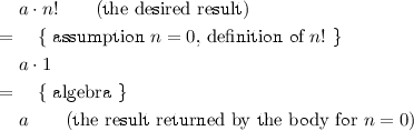
Note that the function header adds some conditions to the contract; in particular, it states the types of the parameters and the result (if any). These are typically checked by the interpreter or compiler. The body of can be verified by distinguishing two cases, and calculating that the desired result is returned.  

Case 1 $\varvec{(n=0){:}}$ :

Case 2 $\varvec{(n \ne 0){:}}$ :

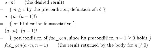
  Note how these two cases correspond to the base and step of an inductive proof.

In fact, we could have started with these calculations before knowing the function’s body, and thereby derive the implementation. That is, contractual reasoning can be used to design (recursive) programs [8, 15, 16]. Bertrand Meyer coined the term design by contract for this approach in 1986 [18, 19].

This approach is so natural that children in primary school, when properly instructed, can successfully apply it [12, 23]. It works best when loops are not introduced, and recursion is the only mechanism available for repeated execution. Of course, you would use different terminology: for every function you must formulate a purpose (its intended effect) and assumptions on when it is supposed to achieve that goal. You need to explain that you can break down problems into problems of the same kind, as long as those new problems are, in some sense, smaller than the original problem.

4.1 Termination of Recursion

That partial correctness is not enough is illustrated by the following function.

It is easy to verify that function satisfies the contract with precondition $True$ and postcondition $False$. Just consider the body, and the contract that it satisfies. Consequently, this function solves all problems, since its precondition is always satisfied, and $False$ implies any other condition. Unfortunately, it does not ‘work’, since it never terminates. But if it would terminate, it would indeed solve all problems. Termination is a separate concern.

Termination of a direct-recursive function f can be argued by providing a variant function, also known as bound function, or just variant, satisfying these conditions:

• 1. the variant function is a mapping

  • from f’s parameters and relevant global variables that satisfy f’s precondition

  • to some well-founded domain (such as the natural numbers, or a subset of the integers that is bounded from below);

• 2. prior to each recursive call of f, the value of the variant function for that call should be strictly less than its value upon entry of f’s body.

In case of the functions , , and , the well-founded domain of the natural numbers suffices, and n can be used as variant function.

When the variant function maps to the natural numbers, its value can serve as an upper bound to the depth of recursion; hence, the name ‘bound function’. This upper bound does not have to be tight; it only concerns termination, and not efficiency. Even if the bound is tight, the runtime and memory complexity can be exponentially higher, as happens to be the case for the naive .

If the recursive function is defined over an inductive type using the bottom-up style (see Subsect. 3.1), then termination is guaranteed, since the inductive type can serve as well-founded domain, and the function’s parameter as variant function.

For functions involving indirect recursion, proving termination is more complex, and beyond the scope of this article.

5 Program Transformations

It can be hard work to design (derive) a program from scratch, even if you ignore efficiency. It would be unfortunate if you had to redesign a program completely to improve its efficiency. This is where program transformations come to the rescue. A correctness-preserving program transformation is a technique that you can apply to a program text to obtain a program that is equivalent, as far as correctness is concerned. Usually the aim of such a transformation is to improve the program in some way, for instance, its performance. There is then no need to redesign it from scratch.

Numerous program transformations are available, in particular also in the area of recursion. We cannot treat them here in any depth. Instead, we will show a couple of examples.

5.1 From Loops to Recursion, and Back

We already mentioned a relationship between loops and recursion in Subsect. 3.2. Every loop can be transformed into an unbounded while-loop, having the form

where represents the local variables initialized by expression , a boolean condition, and and a group of statements. Such a loop can be transformed into the call

of a tail-recursive function defined by

This transformation can also be applied in the other direction: from a tail-recursive function to while-loop. For non- tail-recursive functions there is a similar transformation, as illustrated above with .

It is well-known that any collection of (mutually) recursive functions can be replaced by non-recursive functions and one while-loop, using a stack. The stack holds the intermediate state of each active recursive invocation in a stack frame. At any time, one such invocation is being executed. A recursive call will temporarily suspend execution of the invoking function, and activate a new invocation that will then be executed. When a recursive invocation terminates, its stack frame is popped from the stack, and control returns to its invoker.

Sometimes, such a stack can be implemented simply by an integer variable that is incremented for each new recursive invocation, and decremented when the invocation terminates. Consider, for instance, a function that recognizes whether parentheses in a string are balanced.

5.2 Accumulation Parameters and Continuations for Tail Recursion

A function that is not tail recursive can be transformed into tail recursive form. We have seen that with , which introduced a so-called accumulation parameter (a). In the case of factorial, this generalization is inspired by the calculation for $n\ge 2$:

Compare this to the correctness proof of $fac _{ gen }$ given in Sect. 4. So, in general, we are apparently interested in a calculation of the form

$$\begin{aligned} a \cdot n! \end{aligned}$$

(25)

Thus, we arrive at the generalization $fac _{ gen }(a, n) = a \cdot n!$. Here, a is the accumulation parameter which gathers (accumulates) the final result.

The general transformation takes the following form. Assume that our recursive function looks like this:

This function is not tail recursive, because after the recursive call, function still needs to be applied. If your programming language somehow supports function parameters (and preferably also closures), then we can employ the continuation-passing style (CPS) for generalizing to and to :

where is a type for functions from domain type to range (result) type , and is a function that maps to .

More in detail, is a generic interface in Java defined by

This is a so-called functional interface (introduced in Java 8), which is an interface with just one method.⁶ Any object, say , of any class that implements can serve as a function object, and its function is invoked as .

The expression , where is an expression involving , is a so-called lambda expression (also introduced in Java 8), that provides a compact syntax for defining an object of an anonymous inner class implementing a functional interface.

The resulting function is tail recursive. It pushes all the work that still needs to be done after the original recursive invocation returns, into the continuation parameter , which accumulates an unevaluated composition of deeper and deeper nested calls of : equals . When the base case is encountered, this composition is finally evaluated. Here is our standard factorial function transformed into continuation-passing style:

Now, the call returns factorial. Fortunately, as in the case of factorials, it is often possible to simplify , and replace the passing of a function by the passing of an evaluated expression.

5.3 Tupling

When dealing with multiple functions, on the same arguments, and following the same recursion pattern, these functions can be combined into a single function returning a tuple of the values returned by those functions. This technique is known as tupling [13, 14].

Let’s reconsider the Fibonacci function again, which involves a branching recursion. We can redefine it using two mutually recursive functions:

$$\begin{aligned} fib (0)&= 0 \end{aligned}$$

(26)

$$\begin{aligned} fib (n+1)&= gib (n) \quad \text {for } n\ge 0 \end{aligned}$$

(27)

$$\begin{aligned} gib (0)&= 1 \end{aligned}$$

(28)

$$\begin{aligned} gib (n+1)&= gib (n) + fib (n) \quad \text {for } n\ge 0 \end{aligned}$$

(29)

The functions $fib$ and $gib$ follow the same recursion pattern. Hence, it makes sense to consider the new function $fib\_pair$ defined by

$$\begin{aligned} fib\_pair (n)&= ( fib (n), gib (n)). \end{aligned}$$

(30)

It can be computed recursively, using a 2-element array as pair:

This program has a runtime linear in .

Tupling is a transformation technique dual to accumulation parameters.

6 Recursion Without Recursion in an OO Language

I have occasionally been guilty of telling the following story in introductory programming classes.

      In the beginning, there is data, of various types, and accompanying expressions to operate on data. Variables are used to store data. At each moment in time, a variable has one specific value. Assignment statements modify variables by assigning a value computed from an expression. A selection statement (also known as if-statement) provides conditional execution. All this is relatively easy, but it is still a poor programming formalism: the number of execution steps is bounded by the size of the program.

      Then come loops, a game changer. First bounded loops, with a precomputed upper bound (a.k.a. for-loops), and next unbounded loops (a.k.a. while-loops). Now, program size is no longer an upper bound on program execution: loops can repeatedly execute the same program fragments. This also makes reasoning about programs harder.

      At this point, I tell them that they know all that is needed to program anything that can be computed. The formalism is now universal.

      For convenience (or if you don’t have unbounded integers), we introduce arrays or lists. And also functions, as possibly parameterized abbreviations for program fragments. And when they are ready for it (or not), I introduce them to recursive functions.

      And then I tell them that when you have recursive functions, you can drop the loops, and you still can program everything that is computable. You either need loops or recursion in a programming language to be universal, and both are hard.

Why ‘guilty’? Because the statement ‘You either need loops or recursion in a programming language to be universal’ is not correct. Of course, I know this from Lambda Calculus [27], but that is not imperative programming. Only recently did it dawn upon me how to connect this to object-oriented programming.

Let’s look again at the example of computing factorials. We have already considered generalizations for this problem. Here is another generalization, which we call f. Rather than calling the function itself in the ‘inductive step’, we let it call a function that was provided as argument. That is, we introduce a function parameter, say g (not to be confused with the continuation parameter of Subsect. 5.2):

$$\begin{aligned} f(g, 0)&= 1 \end{aligned}$$

(31)

$$\begin{aligned} f(g, n)&= n \times g(n-1)\quad \text {for } 0 < n \end{aligned}$$

(32)

This function f is not recursive. It does not compute the factorial of n, but does something more general.⁷ If, however, you supply for g any function that computes the factorial (expressible as a pre-post contract for g, which is part of the precondition for f), then f (also) computes the factorial (a postcondition for f):

$$\begin{aligned} (\forall m::g(m) = m!)&\Rightarrow f(g, n) = n! \end{aligned}$$

(33)

Thus, the factorial function $fac$ is a fixed point of f:

$$\begin{aligned} f( fac , n)&= fac (n) \end{aligned}$$

(34)

Using currying,⁸ this can be rewritten as

$$\begin{aligned} f( fac )(n)&= fac (n). \end{aligned}$$

(35)

or even more concisely as

$$\begin{aligned} f( fac )&= fac . \end{aligned}$$

(36)

This might seem to be circular, and therefore pretty useless. But the situation is a bit more subtle. The condition that g should compute the factorial is actually too strong. We can weaken it:

$$\begin{aligned} (\forall m : m < n : g(m) = m!)&\Rightarrow f(g, n) = n! \end{aligned}$$

(37)

(You could weaken it further, because only $m = n-1$ when $0 < n$ is needed. But that is a bit less convenient to formulate, and we don’t need this even weaker condition.)

Now comes the interesting thing. We could use f itself for its own g, if only g would take an additional function parameter. But that is easy to accommodate by ‘upgrading’ the specification of f, so that g takes an extra function parameter:

$$\begin{aligned} f(g, 0)&= 1 \end{aligned}$$

(38)

$$\begin{aligned} f(g, n)&= n \times g(g, n-1)\quad \text {for } 0 < n \end{aligned}$$

(39)

Equation (39) features a self-application of g. We now have the property:

$$\begin{aligned} f(f, n)&= n! \end{aligned}$$

(40)

The proof (omitted) is by induction on n, using (37) for the ‘upgraded’ f:

$$\begin{aligned} (\forall m : m < n : f(f, m) = m!)&\Rightarrow f(f, n) = n! \end{aligned}$$

(41)

6.1 Function Parameters and Self-Application in Java

The Java programming language does allow recursive function definitions. But let’s pretend that these are forbidden. In Subsect. 5.2, we have seen how we can do function parameters in Java, by using an object as ‘carrier’ of a function via an instance method. We define the functional interface :⁹

Here is the code for our generalized factorial function f, using a lambda expression:

This is shorthand for

It is now possible to invoke f(g, n) as . We could invoke this f with as argument for g the identity function id. First, we define this function id by implementing (anonymously) through a lambda expression:

And then test it:¹⁰

It produces as output:

We now invoke f with id as parameter:

This produces as output:

In general, will return $n(n-1)$, except for $n=0$ where it returns 1.

Finally, we invoke f with f as parameter:

obtaining as output:

We could even introduce a type for functions of one argument returning a :

We can then define by

And test it:

To recap, we have defined a non-iterative non-recursive function which we used to define a non-iterative non-recursive function to compute factorials. Of course, there is something loopy: is called repeatedly, because supplies as argument to . This is known as self-application. But this is not a classical ‘static’ recursion, and also not recursive in the data. You could say that has ‘dynamic’ recursion, because it is set up at runtime. To emphasize this even further, we could have defined the factorial function as in the following manner:

Here it is obvious that there is no (static) recursion: since all functions in the definition are anonymous there is no way they can refer to themselves.¹¹

It is a bit unfortunate that you have to pass along this g parameter all of the time, especially since it is always the same function. In the object-oriented setting, we can avoid such copying by putting it in an instance variable, and providing a setter. Instead of an interface, we define an abstract class for this, having an instance variable and providing a setter method :

We now define by

Note how much it resembles the definition of above. We configure and test it as follows:

Now, we do have recursion in the data: the object has obtained a reference to itself via the setter.

6.2 Fixed-Point Combinator in Java

We can generalize this approach further. Suppose you want to define a recursive function $D\rightarrow R$ from domain D to range R without using (static) recursion. We define the generic type for this:

For the recursive calls you introduce a function parameter of the same type $D\rightarrow R$. By currying (see above footnote 2), you define a function $(D\rightarrow R) \rightarrow (D\rightarrow R)$, which is isomorphic to a function with two parameters, one of type $D\rightarrow R$ and another of type D. For this we define the generic type :

For example, for the factorial function, you define

What we still need is a function Y that, when given such a precursor function f, such as , returns its least fixed point. That is, it returns a ‘least’ function r such that

$$\begin{aligned} f(r)&= r. \end{aligned}$$

(42)

Thus, Y must have the property

$$\begin{aligned} f(Y(f))&= Y(f). \end{aligned}$$

(43)

It is tempting try the following recursive definition of method for Y:

But it will not work (it leads to a stack overflow), because the call starts an infinite recursion. Java follows the so-called strict evaluation strategy, where all arguments of a function are evaluated before evaluating the function’s body. We can fix that by a simple trick: delay evaluation of that argument by surrounding it with a lambda abstraction:

In general, a function F is equivalent to $\lambda x. F(x)$. But in Java, a lambda expression is only evaluated when it is supplied with a concrete argument. Therefore, (the body of) the outer application of is now executed first, and it may invoke its argument (the lambda abstraction) if so desired. We now have an indirect self-application of to .

There is also a non-recursive strict way of defining method for Y:

We named it , and it uses self-application based on the function type:

The self-application appears outside . The factorial function is then defined by

In the Lambda Calculus, this fixed-point combinator Y is written concisely as

$$\begin{aligned} Y&= \lambda f. (\lambda x. x(x))(\lambda x. f(\lambda n. x(x)(n))). \end{aligned}$$

(44)

Here, the term $(\lambda x. x(x))$ captures the self-application. If you look carefully, you recognize this structure in the Java code for above. But the Java syntax is still obscuring the beauty of this construction.

Remarks.

• It should be noted that in a formalism like Lambda Calculus, the evaluation of functions, even when defined through a fixed-point combinator, is purely based on substitutions and needs no stack. Nowadays, we would call that self-modifying code.

• It is sobering to realize that the Y-combinator was discovered (invented?) by Haskell Curry long before computing machines existed, possibly as early as 1929 [4]. Alan Turing published his $\varTheta$ fixed-point combinator in 1937.

• Self-application lies at the heart of Gödel’s proof of his famous Incompleteness Theorem.

7 Conclusion

For informatics teachers and anyone who wants to understand more of programming, it is mandatory to know more about recursion. We have presented some key topics for a master class on recursion, thereby highlighting several important aspects of recursion that are often not touched upon in introductory courses.

Important questions both for students and teachers are: What to learn/teach about recursion, and when to do so? The contractual approach explained in Sect. 4 is general, that is, not only applicable to recursive functions, but it is especially helpful in the context of recursion. You cannot go wrong by starting there. For practical programming, the program transformation techniques discussed in Sect. 5 are important. For better theoretical understanding, the preliminaries of Sect. 2, the syntactic and operational view of Sect. 3, and the fixed-point combinator of Sect. 6 are recommended.

The article is not a complete master class on recursion. In particular, more examples and exercises are needed. The following topics were omitted due to space limitations, though they should certainly be included:

• How to nest loops where the nesting depth is controlled by a variable;

• Backtracking, to traverse complex search spaces systematically;

• Dynamic programming, to trade memory and runtime; we recommend [10];

• Branch & bound, to improve performance; see [9] for an abstract approach;

• Recursive descent parsing, to analyze structured texts.

You may have brushed continuation passing (Subsect. 5.2) and fixed-point combinators (Sect. 6) aside as exotic beasts that only appear in the academic world. It is then good to realize that modern programming languages (such as Java) are evolving to incorporate the features underlying these concepts, especially functions as first-class citizens, for a reason. Functional programming is the future. To quote Peyton Jones [21]:

      “If you want to see which features will be in mainstream programming languages tomorrow, then take a look at functional programming languages today. [...]

      Writing software is all about managing complexity, the only thing that limits how ambitious the software that we write is, is really our ability to manage complexity, and functional languages give you much sharper tools for managing complexity than imperative ones do.”