Deterministic Concurrency: A Clock-Synchronised Shared Memory Approach

Abstract

Synchronous Programming (SP) is a universal computational principle that provides deterministic concurrency. The same input sequence with the same timing always results in the same externally observable output sequence, even if the internal behaviour generates uncertainty in the scheduling of concurrent memory accesses. Consequently, SP languages have always been strongly founded on mathematical semantics that support formal program analysis. So far, however, communication has been constrained to a set of primitive clock-synchronised shared memory (csm) data types, such as data-flow registers, streams and signals with restricted read and write accesses that limit modularity and behavioural abstractions.

This paper proposes an extension to the SP theory which retains the advantages of deterministic concurrency, but allows communication to occur at higher levels of abstraction than currently supported by SP data types. Our approach is as follows. To avoid data races, each csm type publishes a policy interface for specifying the admissibility and precedence of its access methods. Each instance of the csm type has to be policy-coherent, meaning it must behave deterministically under its own policy—a natural requirement if the goal is to build deterministic systems that use these types. In a policy-constructive system, all access methods can be scheduled in a policy-conformant way for all the types without deadlocking. In this paper, we show that a policy-constructive program exhibits deterministic concurrency in the sense that all policy-conformant interleavings produce the same input-output behaviour. Policies are conservative and support the csm types existing in current SP languages. Technically, we introduce a kernel SP language that uses arbitrary policy-driven csm types. A big-step fixed-point semantics for this language is developed for which we prove determinism and termination of constructive programs.

1 Introduction

Concurrent programming is challenging. Arbitrary interleavings of concurrent threads lead to non-determinism with data races imposing significant integrity and consistency issues [1]. Moreover, in many application domains such as safety-critical systems, determinism is indeed a matter of life and death. In a medical-device software, for instance, the same input sequence from the sensors (with the same timing) must always result in the same output sequence for the actuators, even if the run-time software architecture regime is unpredictable.

Synchronous programming (SP) delivers deterministic concurrency out of the box¹ which explains its success in the design, implementation and validation of embedded, reactive and safety-critical systems for avionics, automotive, energy and nuclear industries. Right now SP-generated code is flying on the Airbus 380 in systems like flight control, cockpit display, flight warning, and anti-icing just to mention a few. The SP mathematical theory has been fundamental for implementing correct-by-construction program-derivation algorithms and establishing formal analysis, verification and testing techniques [2]. For SCADE², the SP industrial modelling language and software development toolkit, the formal SP background has been a key aspect for its certification at the highest level A of the aerospace standard DO-178B/C. This SP rigour has also been important for obtaining certifications in railway and transportation (EN 50128), industry and energy (IEC 61508), automotive (TÜV and ISO 26262) as well as for ensuring full compliance with the safety standards of nuclear instrumentation and control (IEC 60880) and medical systems (IEC 62304) [3].

Synchronous Programming in a Nutshell. At the top level, we can imagine an SP system as a black-box with inputs and outputs for interacting with its environment. There is a special input, called the clock, that determines when the communication between system and environment can occur. The clock gets an input stimulus from the environment at discrete times. At those moments we say that the clock ticks. When there is no tick, there is no possible communication, as if system and environment were disconnected. At every tick, the system reacts by reading the current inputs and executing a step function that delivers outputs and changes the internal memory. For its part, the environment must synchronise with this reaction and do not go ahead with more ticks. Thus, in SP, we assume (Synchrony Hypothesis) that the time interval of a system reaction, also called macro-step or (synchronous) instant, appears instantaneous (has zero-delay) to the environment. Since each system reaction takes exactly one clock tick, we describe the evolution of the system-environment interaction as a synchronous (lock-step) sequence of macro-steps. The SP theory guarantees that all externally observable interaction sequences derived from the macro-step reactions define a functional input-output relation.

The fact that the sequences of macro-steps take place in time and space (memory) has motivated two orthogonal developments of SP. The data-flow view regards input-output sequences as synchronous streams of data changing over time and studies the functional relationships between streams. Dually, the control-flow approach projects the information of the input-output sequences at each point in time and studies the changes of this global state as time progresses, i.e., from one tick to the next. The SP paradigm includes languages such as Esterel [4], Quartz [5] and SC [6] in the imperative control-flow style and languages like Signal [7], Lustre [8] and Lucid Synchrone [9] that support the declarative data-flow view. There are even mixed control-data flow language such as Esterel V7 [10] or SCADE [3]. Independently of the execution model, the common strength to all of these SP languages is a precise formal semantics—an indispensable feature when dealing with the complexities of concurrency.

At a more concrete level, we can visualise an SP system as a white-box where inside we find (graphical or textual) code. In the SP domain, the program must be divided into fragments corresponding to the macro-step reactions that will be executed instantaneously at each tick. Declarative languages usually organise these macro-steps by means of (internally generated) activation clocks that prescribe the blocks (nodes) that are performed at each tick. Instead, imperative textual languages provide a $\mathop {\mathtt {pause}}$ statement for explicitly delimiting code execution within a synchronous instant. In either case, the Synchrony Hypothesis conveniently abstracts away all the, typically concurrent, low-level micro-steps needed to produce a system reaction. The SP theory explains how the micro-step accesses to shared memory must be controlled so as to ensure that all internal (white-box) behaviour eventually stabilises, completing a deterministic macro-step (black-box) response. For more details on SP, the reader is referred to [2].

State of the Art. Traditional imperative SP languages provide constructs to model control-dominated systems. Typically, these include a concurrent composition of threads (sequential processes) that guarantees determinism and offers signals as the main means for data communication between threads. Signals behave like shared variables for which the concurrent accesses occurring within a macro-step are scheduled according to the following principles: A pure signal has a status that can be present (1) or absent (0). At the beginning of each macro-step, pure signals have status 0 by default. In any instant, a signal ${\texttt {s}}$ can be explicitly emitted with the statement ${\texttt {s}}.\mathop {\mathtt {emit}} ()$ which atomically sets its status to 1. We can read the status of ${\texttt {s}}$ with the statement ${\texttt {s}}.\mathop {\mathtt {pres}} ()$, so the control-flow can branch depending on run-time signal statuses. Specifically, inside programs, if-then-else constructions await for the appropriate combination of present and absent signal statuses to emit (or not) more signals. The main issue is to avoid inconsistencies due to circular causality resulting from decisions based on absent statuses. Thus, the order in which the access methods $\mathop {\mathtt {emit}}$, $\mathop {\mathtt {pres}}$ are scheduled matters for the final result. The usual SP rule for ensuring determinism is that the $\mathop {\mathtt {pres}}$ test must wait until the final signal status is decided. If all signal accesses can be scheduled in this decide-then-read way then the program is constructive. All schedules that keep the decide-then-read order will produce the same input-output result. This is how SP reconciles concurrency and observable determinism and generates much of its algebraic appeal. Constructiveness of programs is what static techniques like the must-can analysis [4, 11,12,13] verify although in a more abstract manner. Pure signals are a simple form of clock-synchronised shared memory (csm) data types with access methods (operations) specific to this csm type. Existing SP control-flow languages also support other restricted csm types such valued signals and arrays [10] or sequentially constructive variables [6].

Contribution. This paper proposes an extension to the SP model which retains the advantages of deterministic concurrency while widening the notion of constructiveness to cover more general csm types. This allows shared-memory communication to occur at higher levels of abstraction than currently supported. In particular, our approach subsumes both the notions of Berry-constructiveness [4] for Esterel and sequential constructiveness for SCL [14]. This is the first time that these SP communication principles are combined side-by-side in a single language. Moreover, our theory permits other predefined communication structures to coexist safely under the same uniform framework, such as data-flow variables [8], registers [15], Kahn channels [16], priority queues, arrays as well as other csm types currently unsupported in SP.

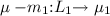
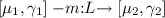
Synopsis and Overview. The core of our approach is presented in Sect. 2 where policies are introduced as a (constructive) synchronisation mechanism for arbitrary abstract data types (ADT). For instance, the policy of a pure signal is depicted in Fig. 1. It has two control states 0 and 1 corresponding to the two possible signal statuses. Transitions are decorated with method names $\mathop {\mathtt {pres}}$, $\mathop {\mathtt {emit}}$ or with $\sigma$ to indicate a clock tick.

Fig. 1.

Pure signal policy.

The policy tells us whether a given method or tick is admissible, i.e., if it can be scheduled from a particular state³. In addition, transitions include a blocking set of method names as part of their action labels. This set determines a precedence between methods from a given state. A label m : L specifies that all methods in L take precedence over m. An empty blocking set $\emptyset$ indicates no precedences. To improve visualisation, we highlight precedences by dotted (red) arrows tagged $\mathop {\mathtt {prec}}$⁴. The policy interface in Fig. 1 specifies the decide-then-read protocol of pure signals as follows. At any instant, if the signal status is 0 then the $\mathop {\mathtt {pres}}$ test can only be scheduled if there are no more potential $\mathop {\mathtt {emit}}$ statements that can still update the status to 1. This explains the precedence of the $\mathop {\mathtt {emit}}$ transition over the self loop with action label $\mathop {\mathtt {pres}} \mathrel {:}\{\mathop {\mathtt {emit}} \}$ from state 0. Conversely, transitions $\mathop {\mathtt {pres}}$ and $\mathop {\mathtt {emit}}$ from state 1 have no precedences, meaning that the $\mathop {\mathtt {pres}}$ and $\mathop {\mathtt {emit}}$ methods are confluent so they can be freely scheduled (interleaved). The reason is that a signal status 1 is already decided and can no longer be changed by either method in the same instant. In general, any two admissible methods that do not block each other must be confluent in the sense that the same policy state is reached independently of their order of execution. Note that all the $\sigma$ transition go to the initial state 0 since at each tick the SP system enters a new macro-step where all pure signals get initialised to the 0 status.

Section 2 describes in detail the idea of a scheduling policy on general csm types. This leads to a type-level coherence property, which is a local form of determinism. Specifically, a csm type is policy-coherent if it satisfies the (policy) specification of admissibility and precedence of its access methods. The point is that a policy-coherent csm type per se behaves deterministically under its own policy—a very natural requirement if the goal is to build deterministic systems that use this type. For instance, the fact that Esterel signals are deterministic (policy-coherent) in the first place permits techniques such as the must-can analysis to get constructive information about deterministic programs. We show how policy-coherence implies a global determinacy property called commutation. Now, in a policy-constructive program all access methods can be scheduled in a policy-conforming way for all the csm types without deadlocking. We also show that, for policy-coherent types, a policy-constructive program exhibits deterministic concurrency in the sense that all policy-conforming interleavings produce the same input-output behaviour.

To implement a constructive scheduling mechanism parameterised in arbitrary csm type policies, we present the synchronous kernel language, called Deterministic Concurrent Language (DCoL), in Sect. 2.1. DCoL is both a minimal language to study the new mathematical concepts but can also act as an intermediate language for compiling existing SP Sect. 3 presents its policy-driven operational semantics for which determinacy and termination is proven. Section 3 also explains how this model generalises existing notions of constructiveness. We discuss related work in Sect. 4 and present our conclusions in Sect. 5.

A companion of this paper is the research report (https://www.uni-bamberg.de/fileadmin/uni/fakultaeten/wiai_professuren/grundlagen_informatik/papersMM/report-WIAI-102-Feb-2018.pdf) [17] which contains detailed proofs and additional examples of csm types.

2 Synchronous Policies

This section introduces a kernel synchronous Deterministic Concurrent Language (DCoL) for policy-conformant constructive scheduling which integrates policy-controlled csm types within a simple syntax. DCoL is used to discuss the behavioural (clock) abstraction limitations of current SP. Then policies are introduced as a mechanism for specifying the scheduling discipline for csm types which, in this form, can encapsulate arbitrary ADTs.

2.1 Syntax

The syntax of DCoL is given by the following operators:

The first two statements correspond to the two forms of immediate completion: $\mathop {\mathtt {skip}}$ terminates instantaneously and $\mathop {\mathtt {pause}}$ waits for the logical clock to terminate. The operators and $P \mathop {{\texttt {;}}} Q$ are parallel interleaving and imperative sequential composition of threads with the standard operational interpretation. Reading and destructive updating is performed through the execution of method calls ${\texttt {c}}.m(e)$ on a csm variable ${\texttt {c}} \in \textsf {O}$ with a method $m \in \textsf {M}_{\texttt {c}}$. The sets $\textsf {O}$ and $\textsf {M}_{\texttt {c}}$ define the granularity of the available memory accesses. The construct $\mathop {{\texttt {let}}} x {{\texttt {\,=\,}}} {\texttt {c}}.m(e) \mathop {{\texttt {in}}} P$ calls m on ${\texttt {c}}$ with an input parameter determined by value expression e. It binds the return value to variable x and then executes program P, which may depend on x, sequentially afterwards. The execution of ${\texttt {c}}.m(e)$ in general has the side-effect of changing the internal memory of ${\texttt {c}}$. In contrast, the evaluation of expression e is side-effect free. For convenience we write $x {{\texttt {\,=\,}}} {\texttt {c}}.m(e) {\mathop {{\texttt {;}}}} P$ for $\mathop {{\texttt {let}}} x {{\texttt {\,=\,}}} {\texttt {c}}.m(e) \mathop {{\texttt {in}}} P$. When P does not depend on x then we write ${\texttt {c}}.m(e){\mathop {{\texttt {;}}}} P$ and ${\texttt {c}}.m(e){\mathop {{\texttt {;}}}}$ for ${\texttt {c}}.m(e){\mathop {{\texttt {;}}}}\mathop {\mathtt {skip}}$. The exact syntax of value expressions e is irrelevant for this work and left open. It could be as simple as permitting only constant value literals or a full-fledged functional language. The conditional $\mathop {\mathtt {{if}}}\, e\, \mathop {\mathtt {then}}\, P\, \mathop {\mathtt {else}}\, P$ has the usual interpretation. For simplicity, we may write $\mathop {\mathtt {{if}}}\, {\texttt {c}}.m(e)\, \mathop {\mathtt {then}}\, P\, \mathop {\mathtt {else}}\, Q$ to mean $x {{\texttt {\,=\,}}} {\texttt {c}}.m(e) {\mathop {{\texttt {;}}}} \mathop {\mathtt {{if}}}\, x\, \mathop {\mathtt {then}}\, P\, \mathop {\mathtt {else}}\, Q$. The recursive closure $\mathop {\textsf {rec}} p.\, P$ binds the behaviour P to the program label p so it can be called from within P. Using this construct we can build iterative behaviours. For instance, ${{\texttt {loop}}} \, P\, {{\texttt {end}}} =_{ \scriptstyle df }\mathop {\textsf {rec}} p.\, P {\mathop {{\texttt {;}}}} \mathop {\mathtt {pause}} {\mathop {{\texttt {;}}}} p$ indefinitely repeats P in each tick. We assume that in a closure $\mathop {\textsf {rec}} p.\, P$ the label p is (i) clock guarded, i.e., it occurs in the scope of at least one $\mathop {\mathtt {pause}}$ (meaning no instantaneous loops) and (ii) all occurrences of p are in the same thread. Thus, $\mathop {\textsf {rec}} p.\, p$ is illegal because of (i) and $\mathop {\textsf {rec}} p.\, (\mathop {\mathtt {pause}} \mathop {{\texttt {;}}} p \mathop {{\texttt {|\!\!|}}}\mathop {\mathtt {pause}} \mathop {{\texttt {;}}} p)$ is not permitted because of (ii).

This syntax seems minimalistic compared to existing SP languages. For instance, it does not provide primitives for pre-emption, suspension or traps as in Quartz or Esterel. Recent work [18] has shown how these control primitives can be translated into the constructs of the SCL language, exploiting destructive update of sequentially constructive (SC) variables. Since SC variables are a special case of policy-controlled csm variables, DCoL is at least as expressive as SCL.

2.2 Limited Abstraction in SP

The pertinent feature of standard SP languages is that they do not permit the programmer to express sequential execution order inside a tick, for destructive updates of signals. All such updates are considered concurrent and thus must either be combined or concern distinct signals. For instance, in languages such as Esterel V7 or Quartz, a parallel composition

$$\begin{aligned} (v {{\texttt {\,=\,}}} {\texttt {xs}}.\textsf {read}() \mathop {{\texttt {;}}} {\texttt {ys}}.\mathop {\mathtt {emit}} (v + 1)) \,\,\mathop {{\texttt {|\!\!|}}}\,\, ({\texttt {xs}}.\mathop {\mathtt {emit}} (1) \mathop {{\texttt {;}}} {\texttt {xs}}.\mathop {\mathtt {emit}} (5)) \end{aligned}$$

(1)

of signal emissions is only constructive if a commutative and associative function is defined on the shared signal ${\texttt {xs}}$ to combine the values assigned to it. But then, by the properties of this combination function, we get the same behaviour if we swap the assignments of values 1 and 5, or execute all in parallel as in

$$\begin{aligned} v {{\texttt {\,=\,}}} {\texttt {xs}}.\textsf {read}() \,\,\mathop {{\texttt {|\!\!|}}}\,\, {\texttt {ys}}.\mathop {\mathtt {emit}} (v + 1) \,\,\mathop {{\texttt {|\!\!|}}}\,\, {\texttt {xs}}.\mathop {\mathtt {emit}} (1) \,\,\mathop {{\texttt {|\!\!|}}}\,\, {\texttt {xs}}.\mathop {\mathtt {emit}} (5). \end{aligned}$$

If what we intended with the second emission ${\texttt {xs}}.\mathop {\mathtt {emit}} (5)$ in (1) was to override the first ${\texttt {xs}}.\mathop {\mathtt {emit}} (1)$ like in normal imperative programming so that the concurrent thread $v {{\texttt {\,=\,}}} {\texttt {xs}}.\textsf {read}() \mathop {{\texttt {;}}} {\texttt {ys}}.\mathop {\mathtt {emit}} (v + 1)$ will read the updated value as $v = 5$? Then we need to introduce a $\mathop {\mathtt {pause}}$ statement to separate the emissions by a clock tick and delay the assignment to ${\texttt {ys}}$ as in

$$\begin{aligned} (\mathop {\mathtt {pause}} \mathop {{\texttt {;}}} v {{\texttt {\,=\,}}} {\texttt {xs}}.\textsf {read}() \mathop {{\texttt {;}}} {\texttt {ys}}.\mathop {\mathtt {emit}} (v + 1)) \,\,\mathop {{\texttt {|\!\!|}}}\,\, ({\texttt {xs}}.\mathop {\mathtt {emit}} (1) \mathop {{\texttt {;}}} \mathop {\mathtt {pause}} \mathop {{\texttt {;}}} {\texttt {xs}}.\mathop {\mathtt {emit}} (5)). \end{aligned}$$

This makes behavioural abstraction difficult. For instance, suppose nats is a synchronous reaction module, possibly composite and with its own internal clocking, which returns the stream of natural numbers. Every time its step function ${{\texttt {nats}}}.{{\texttt {step}}} ()$ is called it returns the next number and increments its internal state. If we want to pair up two successive numbers within one tick of an outer clock and emit them in a single signal ${\texttt {ys}}$ we would write something like $x_1 = {{\texttt {nats}}}.{{\texttt {step}}} () \mathop {{\texttt {;}}} x_2 = {{\texttt {nats}}}.{{\texttt {step}}} () \mathop {{\texttt {;}}} {\texttt {y}}.\mathop {\mathtt {emit}} (x_1, x_2)$ where $x_1$, $x_2$ are thread-local value variables. This over-clocking is impossible in traditional SP because there is no imperative sequential composition by virtue of which we can call the step function of the same module instance twice within a tick. Instead, the two calls ${{\texttt {nats}}}.{{\texttt {step}}} ()$ are considered concurrent and thus create non-determinacy in the value of ${\texttt {y}}$.⁵ To avoid a compiler error we must separate the calls by a clock as in $x_1 = {{\texttt {nats}}}.{{\texttt {step}}} () \mathop {{\texttt {;}}} \mathop {\mathtt {pause}} \mathop {{\texttt {;}}} x_2 = {{\texttt {nats}}}.{{\texttt {step}}} () \mathop {{\texttt {;}}} {\texttt {y}}.\mathop {\mathtt {emit}} (x_1, x_2)$ which breaks the intended clock abstraction.

The data abstraction limitation of traditional SP is that it is not directly possible to encapsulate a composite behaviour on synchronised signals as a shared synchronised object. For this, the simple decide-then-read signal protocol must be generalised, in particular, to distinguish between concurrent and sequential accesses to the shared data structure. A concurrent access $x_1 {{\texttt {\,=\,}}} {{\texttt {nats}}}.{{\texttt {step}}} () \mathop {{\texttt {|\!\!|}}}$ $x_2 {{\texttt {\,=\,}}} {{\texttt {nats}}}.{{\texttt {step}}} ()$ must give the same value for $x_1$ and $x_2$, while a sequential access $x_1 {{\texttt {\,=\,}}} {{\texttt {nats}}}.{{\texttt {step}}} () \mathop {{\texttt {;}}} x_2 {{\texttt {\,=\,}}} {{\texttt {nats}}}.{{\texttt {step}}} ()$ must yield successive values of the stream. In a sequence $x {{\texttt {\,=\,}}} {\texttt {xs}}.{{\texttt {read}}} () \mathop {{\texttt {;}}} {\texttt {xs}}.\mathop {\mathtt {emit}} (v)$ the x does not see the value v but in a parallel we may want the read to wait for the emission. The rest of this section covers our theory on policies in which this is possible. The modularity issue is reconsidered in Sect. 2.6.

2.3 Concurrent Access Policies

In the white-box view of SP, an imperative program consists of a set of threads (sequential processes) and some csm variables for communication. Due to concurrency, a given thread under control (tuc) has the chance to access the shared variables only from time to time. For a given csm variable, a concurrent access policy (cap) is the locking mechanism used to control the accesses of the current tuc and its environment. The locking is to ensure that determinacy of the csm type is not broken by the concurrent accesses. A cap is like a policy which has extra transitions to model potential environment accesses outside the tuc. Concretely, a cap is given by a state machine where each transition label $a \mathrel {:}L$ codifies an action a taking place on the shared variable with blocking set L, where L is a set of methods that take precedence over a. The action is either a method $m \mathrel {:}L$, a silent action $\tau \mathrel {:}L$ or a clock tick $\sigma \mathrel {:}L$. A transition $m \mathrel {:}L$ expresses that in the current cap control state, the method m can be called by the tuc, provided that no method in L is called concurrently. There is a Determinacy Requirement that guarantees that each method call by the tuc has a blocking set and successor state. Additionally, the execution of methods by the cap must be confluent in the sense that if two methods are admissible and do not block each other, then the cap reaches the same policy state no matter the order in which they are executed. This is to preserve determinism for concurrent variable accesses. A transition $\tau \mathrel {:}L$ internalises method calls by the tuc ’s concurrent environment which are uncontrollable for the tuc. In the sequel, the actions in $\textsf {M}_{\texttt {c}} \cup \{\sigma \}$ will be called observable. A transition $\sigma \mathrel {:}L$ models a clock synchronisation step of the tuc. Like method calls, such clock ticks must be determinate as stated by the Determinacy Requirement. Additionally, the clock must always wait for any predicted concurrent $\tau$-activity to complete. This is the Maximal Progress Requirement. Note that we do not need confluence for clock transitions since they are not concurrent.

Definition 1

A concurrent access policy (cap) $\Vdash _{\texttt {c}}$ of a csm variable ${\texttt {c}}$ with (access) methods $\textsf {M}_{\texttt {c}}$ is a state machine consisting of a set of control states $\mathbb {P} _{\texttt {c}}$, an initial state $\varepsilon \in \mathbb {P} _{\texttt {c}}$ and a labelled transition relation $\rightarrow \; \subseteq \mathbb {P} _{\texttt {c}} \times \textsf {A}_{\texttt {c}} \times \mathbb {P} _{\texttt {c}}$ with action labels $\textsf {A}_{\texttt {c}} = (\textsf {M}_{\texttt {c}} \cup \{ \tau , \sigma \}) \times 2^{\textsf {M}_{\texttt {c}}}$. Instead of $(\mu _1, (a, L), \mu _2) \mathop {\in } \rightarrow$ we write . We then say action a is admissible in state $\mu _1$ and blocked by all methods $m \in L \subseteq \textsf {M}_{\texttt {c}}$. When the blocking set L is irrelevant we drop it and write . A cap must satisfy the following conditions:

• Determinacy. If and then $L_1 = L_2$ and $\mu _1 = \mu _2$ provided a is observable, i.e., $a \ne \tau$.

• Confluence. If and do not block each other, i.e., $m_1 \in \textsf {M}_{\texttt {c}} \setminus L_2$ and $m_2 \in \textsf {M}_{\texttt {c}} \setminus L_1$, then for some $\mu '$ both and .

• Maximal Progress.  and  imply a is observable.

A policy is a cap without any (concurrent) $\tau$ activity, i.e., every implies that a is observable. $\square$

Fig. 2.

Synchronous IVar.

The use of a cap as a concurrent policy arises from the notion of enabling. Informally, an observable action $a \in \textsf {M}_{\texttt {c}} \cup \{ \sigma \}$ is enabled in a state $\mu$ of a cap if it is admissible in $\mu$ and in all subsequent states reachable under arbitrary silent steps. To formalise this we define weak transitions $\mu _1 \Rightarrow \mu _2$ inductively to express that either $\mu _1 = \mu _2$ or $\mu _1 \Rightarrow \mu '$ and . We exploit the determinacy for observable actions $a \in \textsf {M}_{\texttt {c}} \cup \{ \sigma \}$ and write $\mu \odot a$ for the unique $\mu '$ such that , if it exists.

Definition 2

Given a cap $\Vdash _{\texttt {c}} = (\mathbb {P} _{\texttt {c}}, \varepsilon , \mathrel {{\mathop {\longrightarrow }\limits ^{}}})$, an observable action $a \in \textsf {M}_{\texttt {c}} \cup \{ \sigma \}$ is enabled in state $\mu \in \mathbb {P} _{\texttt {c}}$, written $\mu \Vdash _{\texttt {c}} \mathop {\downarrow }a$, if $\mu ' \odot a$ exists for all $\mu '$ such that $\mu \Rightarrow \mu '$. A sequence ${{\varvec{a}}} \in (\textsf {M}_{\texttt {c}} \cup \{ \sigma \})^*$ of observable actions is enabled in $\mu \in \mathbb {P} _{\texttt {c}}$, written $\mu \Vdash _{\texttt {c}} \mathop {\downarrow }{{\varvec{a}}}$, if (i) ${{\varvec{a}}} = \varepsilon$ or (ii) ${{\varvec{a}}} = a\, {{\varvec{b}}}$, $\mu \Vdash _{\texttt {c}} \mathop {\downarrow }a$ and $\mu \odot a \Vdash _{\texttt {c}} \mathop {\downarrow }{{\varvec{b}}}$. $\square$

Example 1

Consider the policy $\Vdash _{\texttt {s}}$ in Fig. 1 of an Esterel pure signal ${\texttt {s}}$. An edge labelled a : L from state $\mu _1$ to $\mu _2$ corresponds to a transition in $\Vdash _{\texttt {s}}$. The start state is $\varepsilon = 0$ and the methods $\textsf {M}_{\texttt {s}} = \{ \mathop {\mathtt {pres}}, \mathop {\mathtt {emit}} \}$ are always admissible, i.e., $\mu \odot m$ is defined in each state $\mu$ for all methods m. The presence test does not change the state and any emission sets it to 1, i.e., $\mu \odot \mathop {\mathtt {pres}} = \mu$ and $\mu \odot \mathop {\mathtt {emit}} = 1$ for all $\mu \in \mathbb {P} _{\texttt {s}}$. Each signal status is reset to 0 with the clock tick, i.e., $\mu \odot \sigma = 0$. Clearly, $\Vdash _{\texttt {s}}$ satisfies Determinacy. A presence test on a signal that is not emitted yet has to wait for all pending concurrent emissions, that is $\mathop {\mathtt {emit}}$ blocks $\mathop {\mathtt {pres}}$ in state 0, i.e., . Otherwise, no transition is blocked. Also, all competing transitions and that do not block each other, are of the form $\mu _1 = \mu _2$, from which Confluence follows. Note that since there are no silent transitions, Maximal Progress is always fulfilled too. Moreover, an action sequence is enabled in a state $\mu$ (Definition 2) iff it corresponds to a path in the automaton starting from $\mu$. Hence, for ${{\varvec{m}}} \in \textsf {M}_{\texttt {s}} ^*$ we have $0 \Vdash _{\texttt {s}} \mathop {\downarrow }{{\varvec{m}}}$ iff ${{\varvec{m}}}$ is in the regular language⁶ $\mathop {\mathtt {pres}} ^{*} + \mathop {\mathtt {pres}} ^{*} \mathop {\mathtt {emit}} (\mathop {\mathtt {pres}} + \mathop {\mathtt {emit}})^{*}$ and $1 \Vdash _{\texttt {s}} \mathop {\downarrow }{{\varvec{m}}}$ for all ${{\varvec{m}}} \in \textsf {M}_{\texttt {s}} ^{*}$.

Contrast $\Vdash _{\texttt {s}}$ with the policy $\Vdash _{\texttt {c}}$ of a synchronous immutable variable (IVar) ${\texttt {c}}$ shown in Fig. 2 with methods $\textsf {M}_{\texttt {c}} = \{ {{\texttt {get}}}, {{\texttt {put}}} \}$. During each instant an IVar can be written (put) at most once and cannot be read (get) until it has been written. No value is stored between ticks, which means the memory is only temporary and can be reused, e. g., IVars can be implemented by wires. Formally, $\mu \Vdash _{\texttt {c}} \mathop {\downarrow }{{\texttt {put}}}$ iff $\mu = 0$, where 0 is the initial empty state and $\mu \Vdash _{\texttt {c}} \mathop {\downarrow }{{\texttt {get}}}$ iff $\mu = 1$, where 1 is the filled state. The transition switches to filled state where get is admissible but put is not, anymore. The blocking $\{ {{\texttt {put}}} \}$ means there cannot be other concurrent threads writing ${\texttt {c}}$ at the same time.    $\square$

2.4 Enabling and Policy Conformance

A policy describes what a single thread can do to a csm variable ${\texttt {c}}$ when it operates alone. In a cap all potential activities of the environment are added as $\tau$-transitions to block the tuc ’s accesses. To implement this $\tau$-locking we define an operation that generates a cap $[\mu , \gamma ]$ out of a policy. In this construction, $\mu \in \mathbb {P} _{\texttt {c}}$ is a policy state recording the history of methods that have been performed on ${\texttt {c}}$ so far ($must$ information). The second component $\gamma \subseteq \textsf {M}_{\texttt {c}} ^*$ is a prediction for the sequences of methods that can still potentially be executed by the concurrent environment ($can$ information).

Definition 3

Let $(\mathbb {P} _{\texttt {c}}, \varepsilon , \rightarrow )$ be a policy. We define a cap $\Vdash _{\texttt {c}}$ where states are pairs $[\mu , \gamma ]$ such that $\mu \in \mathbb {P} _{\texttt {c}}$ is a policy state and $\gamma \subseteq \textsf {M}_{\texttt {c}} ^*$ is a prediction. The initial state is $[\varepsilon , \textsf {M}_{\texttt {c}} ^*]$ and the transitions are as follows:

• 1. The observable transitions are such that $\gamma _1 = \gamma _2$ and 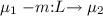provided that for all sequences $n\,{{\varvec{n}}} \in \gamma _1$ with we have $n \not \in L$.

• 2. The silent transitions are such that $\emptyset \ne m\, \gamma _2 \subseteq \gamma _1$ and .

• 3. The clock transitions are such that $\gamma _1 = \emptyset$ and .    $\square$

Silent steps arise from the concurrent environment: A step removes some prefix method m from the environment prediction $\gamma _1$, which contracts to an updated suffix prediction $\gamma _2$ with $m\, \gamma _2 \subseteq \gamma _1$. This method m is executed on the csm variable, changing the policy state to $\mu _2 = \mu _1 \odot m$. A method m is enabled, $[\mu , \gamma ] \Vdash _{\texttt {c}} \mathop {\downarrow }m$, if for all $[\mu _1, \gamma _1]$ which are $\tau$-reachable from $[\mu , \gamma ]$, method m is admissible, i.e., for some $\mu _2$.

Example 2

Consider concurrent threads , where $P_2 = {\texttt {zs}}.{{{\texttt {put}}} (5)} \mathop {{\texttt {;}}} u {{\texttt {\,=\,}}}$ ${\texttt {ys}}.{{{\texttt {get}}}}()$ and $P_1 = v {{\texttt {\,=\,}}} {\texttt {zs}}.{{{\texttt {get}}}}() \mathop {{\texttt {;}}} {\texttt {ys}}.{{\texttt {put}}} (v+1)$ with IVars ${\texttt {zs}}$, ${\texttt {ys}}$ according to Example 1. Under the IVar policy the execution is deterministic, so that first $P_2$ writes on ${\texttt {zs}}$, then $P_1$ reads from ${\texttt {zs}}$ and writes to ${\texttt {ys}}$, whereupon finally $P_1$ reads ${\texttt {ys}}$. Suppose the variables have reached policy states $\mu _{\texttt {zs}}$ and $\mu _{\texttt {ys}}$ and the threads are ready to execute the residual programs $P_i'$ waiting at some method call ${\texttt {c}} _i.m_i(v_i)$, respectively. Since thread $P_i'$ is concurrent with the other $P_{3-i}'$, it can only proceed if $m_i$ is not blocked by $P_{3-i}'$, i.e., if $[\mu _{{\texttt {c}} _i}, can _{{\texttt {c}} _i}(P_{3-i}') ] \Vdash _{{\texttt {c}} _i} \mathop {\downarrow }m_i$, where $can _{{\texttt {c}}}(P) \subseteq \textsf {M}_{\texttt {c}} ^*$ is the set of method sequences predicted for P on ${\texttt {c}}$.

Initially we have $\mu _{\texttt {zs}} = 0 = \mu _{\texttt {ys}}$. Since method ${{\texttt {get}}}$ is not admissible in state 0, we get $[0, can _{{\texttt {zs}}}(P_{2}) ] \nVdash _{{\texttt {zs}}} \mathop {\downarrow }{{\texttt {get}}}$ by Definitions 3 and 2. So, $P_1$ is blocked. The ${\texttt {zs}}.{{\texttt {put}}}$ of $P_2$, however, can proceed. First, since no predicted method sequence $can _{{\texttt {zs}}}(P_{1}) = \{ {{\texttt {get}}} \}$ of $P_1$ starts with ${{\texttt {put}}}$, the transition implies that by Definition 3(1). Moreover, since get of $P_1$ is not admissible in 0, there are no silent transitions out of $[0, can _{{\texttt {zs}}}(P_{1}) ]$ according to Definition 3(2). Thus, $[0, can _{{\texttt {zs}}}(P_{1}) ] \Vdash _{\texttt {zs}} \mathop {\downarrow }{{\texttt {put}}}$, as claimed.

When the ${\texttt {zs}}.{{\texttt {put}}}$ is executed by $P_2$ it turns into $P_2' = u {{\texttt {\,=\,}}} {\texttt {ys}}.{{\texttt {get}}} ()$ and the policy state for ${\texttt {zs}}$ advances to $\mu _{\texttt {zs}} ' = 1$, while ${\texttt {ys}}$ is still at $\mu _{\texttt {ys}} = 0$. Now ${\texttt {ys}}.{{\texttt {get}}}$ of $P_2'$ blocks for the same reason as ${\texttt {zs}}$ was blocked in $P_1$ before. But since $P_2$ has advanced, its prediction on ${\texttt {zs}}$ reduces to $can _{{\texttt {zs}}}(P_2') = \emptyset$. Therefore, the transition implies by Definition 3(1). Also, there are no silent transitions out of $[1, can _{{\texttt {zs}}}(P_2') ]$ by Definition 3(2) and so $[\mu _{\texttt {zs}} ', can _{{\texttt {zs}}}(P_2') ] \Vdash _{\texttt {zs}} \mathop {\downarrow }{{\texttt {get}}}$ by Definition 2. This permits $P_1$ to execute ${\texttt {zs}}.{{\texttt {get}}} ()$ and proceed to $P_1' = {\texttt {ys}}.{{\texttt {put}}} (5+1)$. The policy state of ${\texttt {zs}}$ is not changed by this, neither is the state of ${\texttt {ys}}$, whence $P_2'$ is still blocked. Yet, we have $[\mu _{\texttt {ys}}, can _{{\texttt {zs}}}(P_2') ] \Vdash _{\texttt {ys}} \mathop {\downarrow }{{\texttt {put}}}$ which lets $P_1'$ complete ${\texttt {ys}}.{{\texttt {put}}}$. It reaches $P_1''$ with $can _{{\texttt {ys}}}(P_1'') = \emptyset$ and changes the policy state of ${\texttt {ys}}$ to $\mu _{\texttt {ys}} ' = 1$. At this point, $[\mu _{\texttt {ys}} ', can _{{\texttt {zs}}}(P_1'') ] \Vdash _{\texttt {ys}} \mathop {\downarrow }{{\texttt {get}}}$ which means $P_2'$ unblocks to execute ${\texttt {ys}}.{{\texttt {get}}}$.    $\square$

Definition 4

Let $\Vdash _{\texttt {c}}$ be a policy for ${\texttt {c}}$. A method sequence ${{\varvec{m}}}_{1}$ blocks another ${{\varvec{m}}}_{2}$ in state $\mu$, written $\mu \Vdash _{\texttt {c}} {{\varvec{m}}}_{1} \rightarrow {{\varvec{m}}}_{2}$, if $\mu \Vdash _{\texttt {c}} \mathop {\downarrow }{{\varvec{m}}}_{2}$ but $[\mu , \{ {{\varvec{m}}}_{1} \}] \nVdash _{\texttt {c}} \mathop {\downarrow }{{\varvec{m}}}_{2}$. Two method sequences ${{\varvec{m}}}_{1}$ and ${{\varvec{m}}}_{2}$ are concurrently enabled, denoted $\mu \Vdash _{\texttt {c}} {{\varvec{m}}}_{1} \mathrel {\diamond _{}} {{\varvec{m}}}_{2}$ if $\mu \Vdash _{\texttt {c}} \mathop {\downarrow }{{\varvec{m}}}_{1}$, $\mu \Vdash _{\texttt {c}} \mathop {\downarrow }{{\varvec{m}}}_{2}$ and both $\mu \nVdash _{\texttt {c}} {{\varvec{m}}}_{1} \rightarrow {{\varvec{m}}}_{2}$ and $\mu \nVdash _{\texttt {c}} {{\varvec{m}}}_{2} \rightarrow {{\varvec{m}}}_{1}$.    $\square$

Our operational semantics will only let a tuc execute a sequence ${{\varvec{m}}}$ provided $[\mu , \gamma ] \Vdash _{\texttt {c}} \mathop {\downarrow }{{\varvec{m}}}$, where $\mu$ is the current policy state of ${\texttt {c}}$ and $\gamma$ the predicted activity in the tuc ’s concurrent environment. Symmetrically, the environment will execute any ${{\varvec{n}}} \in \gamma$ only if it is enabled with respect to ${{\varvec{m}}}$, i.e., if $[\mu , \{{{\varvec{m}}}\}] \Vdash \mathop {\downarrow }{{\varvec{n}}}$. This means $\mu \Vdash _{\texttt {c}} {{\varvec{m}}} \mathrel {\diamond _{}} {{\varvec{n}}}$. Policy coherence (Definition 5 below) then implies that every interleaving of the sequences ${{\varvec{m}}}$ and any ${{\varvec{n}}} \in \gamma$ leads to the same return values and final variable state (Proposition 1).

2.5 Coherence and Determinacy

A method call m(v) combines a method $m \in \textsf {M}_{\texttt {c}}$ with a method parameter⁷ $v \in \mathbb {D}$, where $\mathbb {D}$ is a universal domain for method arguments and return values, including the special don’t care value ${\_} \in \mathbb {D}$. We denote by $\textsf {A}_{\texttt {c}} = \{ m(v) \mid m \in \textsf {M}_{\texttt {c}}, v \in \mathbb {D} \}$ the set of all method calls on object ${\texttt {c}}$. Sequences of method calls $\alpha \in \textsf {A}_{\texttt {c}} ^*$ can be abstracted back into sequences of methods $\alpha ^\# \in \textsf {M}_{\texttt {c}} ^*$ by dropping the method parameters: $\varepsilon ^\# = \varepsilon$ and $(m(v)\, \alpha )^\# = m\, \alpha ^\#$.

Coherence concerns the semantics of method calls as state transformations. Let $\mathbb {S} _{\texttt {c}}$ be the domain of memory states of the object ${\texttt {c}}$ with initial state $init _{\texttt {c}} \in \mathbb {S} _{\texttt {c}}$. Each method call $m(v) \in \textsf {A}_{\texttt {c}}$ corresponds to a semantical action $[\![m(v)]\!]_{\texttt {c}} \in \mathbb {S} _{\texttt {c}} \rightarrow (\mathbb {D} \times \mathbb {S} _{\texttt {c}})$. If $s \in \mathbb {S} _{\texttt {c}}$ is the current state of the object then executing a call m(v) on ${\texttt {c}}$ returns a pair $(u, s') = [\![m(v)]\!]_{\texttt {c}} (s)$ where the first projection $u \in \mathbb {D}$ is the return value from the call and the second projection $s' \in \mathbb {S} _{\texttt {c}}$ is the new updated state of the variable. For convenience, we will denote $u = \pi _1 [\![m(v)]\!]_{\texttt {c}} (s)$ by $u = s.m(v)$ and $s' = \pi _2[\![m(v)]\!]_{\texttt {c}} (s)$ by $s' = s \odot m(v)$. The action notation is extended to sequences of calls $\alpha \in \textsf {A}_{\texttt {c}} ^*$ in the natural way: $s \odot \varepsilon = s$ and $s \odot (m(v)\,\alpha ) = (s \odot m(v)) \odot \alpha$.

For policy-based scheduling we assume an abstraction function mapping a memory state $s \in \mathbb {S} _{\texttt {c}}$ into a policy state $s^\# \in \mathbb {P} _{\texttt {c}}$. Specifically, $init _{\texttt {c}} ^\# = \varepsilon$. Further, we assume the abstraction commutes with method execution in the sense that if we execute a sequence of calls and then abstract the final state, we get the same as if we executed the policy automaton on the abstracted state in the first place. Formally, $(s \odot \alpha )^\# = s^\# \odot \alpha ^\#$ for all $s \in \mathbb {S} _{\texttt {c}}$ and $\alpha \in A_{\texttt {c}} ^*$.

Definition 5

(Coherence). A csm variable ${\texttt {c}}$ is policy-coherent if for all method calls $a, b \in \textsf {A}_{\texttt {c}}$ whenever $s^\# \Vdash _{\texttt {c}} a^\# \mathrel {\diamond _{}} b^\#$ for a state $s \in \mathbb {S} _{\texttt {c}}$, then a and b are confluent in the sense that $s.a = (s \odot b).a$, $s.b = (s \odot a).b$ and $s \odot a \odot b = s \odot b \odot a$.    $\square$

Example 3

Esterel pure signals do not carry any data value, so their memory state coincides with the policy state, $\mathbb {S} _{\texttt {s}} = \mathbb {P} _{\texttt {s}} = \{ 0, 1 \}$ and $s^\# = s$. An emission $\mathop {\mathtt {emit}}$ does not return any value but sets the state of ${\texttt {s}}$ to 1, i.e., $s.\mathop {\mathtt {emit}} ( {\_} ) = {\_} \in \mathbb {D}$ and ${s}{\odot }{\mathop {\mathtt {emit}} ( {\_} ) = 1 \in \mathbb {S} _{\texttt {s}}}$. A present test returns the state, $s.\mathop {\mathtt {pres}} ( {\_} ) = s$, but does not modify it, ${s}{\odot }{\mathop {\mathtt {pres}} ( {\_} ) = s}$. From the policy Fig. 1 we find that the concurrent enablings $s^\# \Vdash _{\texttt {s}} a^\# \mathrel {\diamond _{}} b^\#$ according to Definition 4 are (i) $a = b \in \{ \mathop {\mathtt {pres}} ( {\_} ), \mathop {\mathtt {emit}} ( {\_} ) \}$ for arbitrary s, or (ii) $s = 1$, $a = \mathop {\mathtt {emit}} ( {\_} )$ and $b = \mathop {\mathtt {pres}} ( {\_} )$. In each of these cases we verify $s.a = (s \odot b).a$, $s.b = (s \odot a).b$ and $s \odot a \odot b = s \odot b \odot a$ without difficulty. Note that $1 \Vdash _{\texttt {s}} \mathop {\mathtt {emit}} \mathrel {\diamond _{}} \mathop {\mathtt {pres}}$ since the order of execution is irrelevant if $s = 1$. On the other hand, $0 \nVdash _{\texttt {s}} \mathop {\mathtt {emit}} \mathrel {\diamond _{}} \mathop {\mathtt {pres}}$ because in state 0 both methods are not confluent. Specifically, $0.\mathop {\mathtt {pres}} ( {\_} ) = 0 \ne 1 = (0 \odot \mathop {\mathtt {emit}} ( {\_} )).\mathop {\mathtt {pres}} ( {\_} )$.    $\square$

A special case are linear precedence policies where $\mu \Vdash _{\texttt {c}} \mathop {\downarrow }m$ for all $m \in \textsf {M}_{\texttt {c}}$ and $\mu \Vdash _{\texttt {c}} m \rightarrow n$ is a linear ordering on $\textsf {M}_{\texttt {c}}$, for all policy states $\mu$. Then, for no state we have $\mu \Vdash _{\texttt {c}} m_{1} \mathrel {\diamond _{}} m_2$, so there is no concurrency and thus no confluence requirement to satisfy at all. Coherence of ${\texttt {c}}$ is trivially satisfied whatever the semantics of method calls. For any two admissible methods one takes precedence over the other and thus the enabling relation becomes deterministic. There is however a risk of deadlock which can be excluded if we assume that threads always call methods in order of decreasing precedence.

The other extreme case is where the policy makes all methods concurrently enabled, i.e., $\mu \Vdash _{\texttt {c}} m_1 \mathrel {\diamond _{}} m_2$ for all policy states $\mu$ and methods $m_1$, $m_2$. This avoids deadlock completely and gives maximal concurrency but imposes the strongest confluence condition, viz. independently of the scheduling order of any two methods, the resulting variable state must be the same. This requires complete isolation of the effects of any two methods. Such an extreme is used, e. g., in the CR library [19]. The typical csm variable, however, will strike a trade-off between these two extremes. It will impose a sensible set of precedences that are strong enough to ensure coherent implementations and thus determinacy for policy-conformant scheduling, while at the same time being sufficiently relaxed to permit concurrent implementations and avoiding unnecessary deadlocks risking that programs are rejected by the compiler as un-scheduleable.

Whatever the policies, if the variables are coherent, then all policy-conformant interleavings are indistinguishable for each csm variable. To state schedule invariance in its general form we lift method actions and independence to multi-variable sequences of methods calls $\textsf {A} = \{ {\texttt {c}}.m(v) \mid {\texttt {c}} \in \textsf {O}, m(v) \in \textsf {A}_{\texttt {c}} \}$. For a given sequence $\alpha \in \textsf {A}^*$ let $\pi _{\texttt {c}} (\alpha ) \in \textsf {A}_{\texttt {c}} ^*$ be the projection of $\alpha$ on ${\texttt {c}}$, formally $\pi _{\texttt {c}} (\varepsilon ) = \varepsilon$, $\pi _{\texttt {c}} ({\texttt {c}}.m(v)\, \alpha ) = m(v)\, \pi _{\texttt {c}} (\alpha )$ and $\pi _{\texttt {c}} ({\texttt {c}} '.m(v)\, \alpha ) = \pi _{\texttt {c}} (\alpha )$ for ${\texttt {c}} ' \ne {\texttt {c}}$. A global memory ${\varSigma } \in \mathbb {S} = \prod _{{\texttt {c}} \in \textsf {O}} \mathbb {S} _{\texttt {c}}$ assigns a local memory ${\varSigma }.{\texttt {c}} \in \mathbb {S} _{\texttt {c}}$ to each variable ${\texttt {c}}$. We write $init$ for the initial memory that has $init .{\texttt {c}} = init _{\texttt {c}}$ and $( init .{\texttt {c}})^\# = \varepsilon \in \mathbb {P} _{\texttt {c}}$.

Given a global memory ${\varSigma } \in \mathbb {S}$ and sequences $\alpha , \beta \in \textsf {A}^*$ of method calls, we extend the independence relation of Definition 4 variable-wise, defining ${\varSigma } \Vdash \alpha \mathrel {\diamond _{}} \beta$ iff $({\varSigma }.{\texttt {c}})^\# \Vdash _{\texttt {c}} (\pi _{\texttt {c}} (\alpha ))^\# \mathrel {\diamond _{}} (\pi _{\texttt {c}} (\beta ))^\#$. The application of a method call $a \in \textsf {A}$ to a memory ${\varSigma } \in \mathbb {S}$ is written ${\varSigma }.a \in \mathbb {S}$ and defined $({\varSigma }.({\texttt {c}}.m(v))).{\texttt {c}} = ({\varSigma }.{\texttt {c}}).m(v)$ and $({\varSigma }.({\texttt {c}}.m(v))).{\texttt {c}} ' = {\varSigma }.{\texttt {c}} '$ for ${\texttt {c}} ' \ne {\texttt {c}}$. Analogously, method actions are lifted to global memories, i.e., $({\varSigma } \odot {\texttt {c}}.m(v)).{\texttt {c}} ' = {\varSigma }.{\texttt {c}} '$ if ${\texttt {c}} ' \ne {\texttt {c}}$ and $({\varSigma } \odot {\texttt {c}}.m(v)).{\texttt {c}} = {\varSigma }.{\texttt {c}} \odot m(v)$.

Proposition 1

(Commutation). Let all csm variables be policy-coherent and ${\varSigma } \Vdash a\mathrel {\diamond _{}} \alpha$ for a memory ${\varSigma } \in \mathbb {S}$, method call $a \in \textsf {V}$ and sequences of method calls $\alpha \in \textsf {V}^*$. Then, ${\varSigma } \odot a \odot \alpha = {\varSigma } \odot \alpha \odot a$ and ${\varSigma }.a = ({\varSigma } \odot \alpha ).a$.

2.6 Policies and Modularity

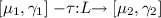
Consider the synchronous data-flow network cnt in Fig. 3b with three process nodes, a multiplexer mux, a register reg and an incrementor inc. Their DCoL code is given in Fig. 3a. The network implements a settable counter, which produces at its output ${\texttt {ys}}$ a stream of consecutive integers, incremented with each clock tick. The wires ${\texttt {ys}}$, ${\texttt {zs}}$ and ${\texttt {ws}}$ are IVars (see Example 2) carrying a single integer value per tick. The input ${\texttt {xs}}$ is a pure Esterel signal (see Example 1). The counter state is stored by reg in a local variable xv with ${{\texttt {read}}}$ and ${{\texttt {write}}}$ methods that can be called by a single thread only. The register is initialised to value 0 and in each subsequent tick the value at ${\texttt {ys}}$ is stored. The inc takes the value at ${\texttt {zs}}$ and increments it. When the signal ${\texttt {xs}}$ is absent, mux passes the incremented value on ${\texttt {ws}}$ to ${\texttt {ys}}$ for the next tick. Otherwise, if ${\texttt {xs}}$ is present then mux resets ${\texttt {ys}}$.

The evaluation order is implemented by the policies of the IVars ${\texttt {ys}}$, ${\texttt {zs}}$ and ${\texttt {ws}}$. In each case the put method takes precedence over get which makes sure that the latter is blocked until the former has been executed. The causality cycle of the feedback loop is broken by the fact that the reg node first sends the current counter value to ${\texttt {zs}}$ before it waits for the new value at ${\texttt {ys}}$. The other nodes mux and inc, in contrast, first read their inputs and then send to their output.

Fig. 3.

Synchronous data-flow network cnt built from control-flow processes.

Now suppose, for modularity, the reg node is pre-compiled into a synchronous IO automaton to be used by mux and inc as a black box component. Then, ${{\texttt {reg}}}$ must be split into three modes [20] ${{\texttt {reg}}}.{{\texttt {init}}}$, ${{\texttt {reg}}}.{{\texttt {get}}}$ and ${{\texttt {reg}}}.{{\texttt {set}}}$ that can be called independently in each instant. The init mode initialises the register memory with 0. The ${{\texttt {get}}}$ mode extracts the buffered value and ${{\texttt {set}}}$ stores a new value into the register. Since there may be data races if get and set are called concurrently on reg, a policy must be imposed. In the scheduling of Fig. 3b, first ${{\texttt {reg}}}.{{\texttt {get}}}$ is executed to place the output on ${\texttt {zs}}$. Then, ${{\texttt {reg}}}$ waits for ${{\texttt {mux}}}$ to produce the next value of ${\texttt {ys}}$ from ${\texttt {xs}}$ or ${\texttt {ws}}$. Finally, ${{\texttt {reg}}}.{{\texttt {set}}}$ is executed to store the current value of ${\texttt {ys}}$ for the next tick. Thus, the natural policy for the register is to require that in each tick set is called by at most one thread and if so no concurrent call to get by another thread happens afterwards. In addition, the policy requires init to take place at least once before any set or get. Hence, the policy has two states $\mathbb {P} _{{\texttt {reg}}} = \{ 0, 1 \}$ with initial $\varepsilon = 0$ and admissibility such that $0 \Vdash _{{\texttt {reg}}} \mathop {\downarrow }m$ iff $m = {{\texttt {init}}}$ and $1 \Vdash _{{\texttt {reg}}} \mathop {\downarrow }m$ for all m. The transitions are $0 \odot {{\texttt {init}}} = 1$ and $1 \odot m = 1$ for all $m \in \textsf {M}_{{\texttt {reg}}}$. Further, for coherence, in state 1 no set may be concurrent and every get must take place before any concurrent set. This means, we have $1 \Vdash _{{{\texttt {reg}}}} m \rightarrow {{\texttt {set}}}$ for all $m \in \{ {{\texttt {get}}}, {{\texttt {set}}} \}$. Figure 3c shows the partially compiled code in which reg is treated as a compiled object. The policy on reg makes sure the accesses by mux and inc are scheduled in the right way (see Example 4). Note that reg is not an IVar because it has memory.

The cnt example exhibits a general pattern found in the modular compilation of SP: Modules (here reg) may be exercised several times in a synchronous tick through modes which are executed in a specific prescribed order. Mode calls (here ${{\texttt {reg}}}.{{\texttt {set}}}$, ${{\texttt {reg}}}.{{\texttt {get}}}$) in the same module are coupled via common shared memory (here the local variable ${\texttt {xs}}$) while mode calls in distinct modules are isolated from each other [15, 20].

3 Constructive Semantics of DCoL

To formalise our semantics it is technically expedient to keep track of the completion status of each active thread inside the program expression. This results in a syntax for processes distinguished from programs in that each parallel composition is labelled by completion codes $k_i \in \{ \bot , 0, 1 \}$ which indicate whether each thread is waiting $k_i = \bot$, terminated 0 or pausing $k_i = 1$. Since we remove a process from the parallel as soon as it terminates then the code $k_i = 0$ cannot occur. An expression is considered a special case of a process with $k_i = \bot$. The formal semantics is given by a reduction relation on processes

(2)

specified by the inductive rules in Figs. 4 and 5. The relation (2) determines an instantaneous sequential reduction step of process P, called an sstep, that follows a sequence of enabled method calls ${{\varvec{m}}} \in \textsf {M}^*$ in sequential program order in P. This does not include any context switches between concurrent threads inside P. For thread communication, several ssteps must be chained up, as described later. The sstep (2) results in an updated memory ${\varSigma } '$ and residual process $P'$. The subscript $k'$ is a completion code, described below. The reduction (2) is performed in a context consisting of a global memory ${\varSigma } \in \mathbb {S}$ ($must$ context) containing the current state of all csm variables and an environment prediction $\varPi \subseteq \textsf {M}^*$ ($can$ context). The prediction records all potentially outstanding methods sequences from threads running concurrently with P.

We write $\pi _{\texttt {c}} ({{\varvec{m}}}) \in \textsf {M}_{\texttt {c}} ^*$ for the projection of a method sequence ${{\varvec{m}}} \in \textsf {M}^*$ to variable ${\texttt {c}}$ and write $\pi _{\texttt {c}} (\varPi )$ for its lifting to sets of sequences. Prefixing is lifted, too, i.e., ${\texttt {c}}.m \odot \varPi = \{ {\texttt {c}}.m\, {{\varvec{m}}} \mid {\varvec{m}} \in \varPi \}$ for any ${\texttt {c}}.m \in \textsf {M}$.

Performing a method call ${\texttt {c}}.m(v)$ in ${\varSigma }; \varPi$ advances the $must$ context to ${\varSigma } \odot {\texttt {c}}.m(v)$ but leaves $\varPi$ unchanged. The sequence of methods ${{\varvec{m}}} \in \textsf {M}^*$ in (2) is enabled in ${\varSigma }; \varPi$, written $[{\varSigma }, \varPi ] \Vdash \mathop {\downarrow }{{\varvec{m}}}$ meaning that $[({\varSigma }.{\texttt {c}})^\#, \pi _{\texttt {c}} (\varPi )] \Vdash _{\texttt {c}} \mathop {\downarrow }\pi _{\texttt {c}} ({{\varvec{m}}})$ for all ${\texttt {c}} \in \textsf {O}$. In this way, the context $[{\varSigma }, \varPi ]$ forms a joint policy state for all variables for the tuc P, in the sense of Sect. 2 (Definition 3).

Fig. 4.

SStep reductions for sequence, completion and recursion.

Fig. 5.

SStep reductions for method calls, conditional and parallel.

Fig. 6.

Computing the $can$ prediction.

Most of the rules in Figs. 4 and 5 should be straightforward for the reader familiar with structural operational semantics. $\textsf {Seq} _1$ is the case of a sequential P; Q where P pauses or waits ($k' \ne 0$) and $\textsf {Seq} _2$ is where P terminates and control passes into Q. The statements $\mathop {\mathtt {skip}}$ and $\mathop {\mathtt {pause}}$ are handled by rules $\textsf {Cmp} _1$ and $\textsf {Cmp} _2$. The rule $\textsf {Rec}$ explains recursion $\mathop {\textsf {rec}} p. P$ by syntactic unfolding of the recursion body P. All interaction with the memory takes place in the method calls $\mathop {{\texttt {let}}} x = {\texttt {c}}.m(e)\; \mathop {{\texttt {in}}} P$. Rule $\textsf {Let} _1$ is applicable when the method call is enabled, i.e., $[{\varSigma }, \varPi ] \Vdash \mathop {\downarrow }{\texttt {c}}.m$. Since processes are closed, the argument expression e must evaluate, $eval (e) = v$, and we obtain the new memory ${\varSigma } \odot {\texttt {c}}.m(v)$ and return value ${\varSigma }.{\texttt {c}}.m(v)$. The return value is substituted for the local (stack allocated) identifier x, giving the continuation process $P\{{\varSigma }.{\texttt {c}}.m(v)/x\}$ which is run in the updated context ${\varSigma } \odot {\texttt {c}}.m(v); \varPi$. The prediction $\varPi$ remains the same. The second rule $\textsf {Let} _2$ is used when the method call is blocked or the thread wants to wait and yield to the scheduler. The rules for conditionals $\textsf {Cnd} _1$, $\textsf {Cnd} _2$ are canonical. More interesting are the rules $\textsf {Par} _1$–$\textsf {Par} _4$ for parallel composition, which implement non-deterministic thread switching. It is here where we need to generate predictions and pass them between the threads to exercise the policy control.

The key operation is the computation of the $can$-prediction of a process P to obtain an over-approximation of the set of possible method sequences potentially executed by P. For compositionality we work with sequences $can ^s(P) \subseteq \textsf {M}^*\times \{ 0 , 1 \}$ stoppered with a completion code 0 if the sequence ends in termination or 1 if it ends in pausing. The symbols $\bot _0$, $\bot _1$ and $\top$ are the terminated, paused and fully unconstrained $can$ contexts, respectively, with $\bot _0 = \{ (\varepsilon , 0) \}$, $\bot _1 = \{ (\varepsilon , 1) \}$ and $\top = \textsf {M}^*\times \{ 0 , 1 \}$. The set $can ^s(P)$, defined in Fig. 6, is extracted from the structure of P using prefixing ${\texttt {c}}.m \odot \varPi '$, choice $\varPi _1' \oplus \varPi _2' = \varPi _1' \cup \varPi _2'$, parallel $\varPi _1' \otimes \varPi _2'$ and sequential composition $\varPi _1' \cdot \varPi _2'$. Sequential composition is obtained pairwise on stoppered sequences such that $({{\varvec{m}}}, 0) \cdot ({{\varvec{n}}}, c) = ({{\varvec{m}}}\, {\varvec{n}}, c)$ and $({{\varvec{m}}}, 1) \cdot ({{\varvec{n}}}, c) = ({{\varvec{m}}}, 1)$. As a consequence, $\bot _0 \cdot \varPi ' = \varPi '$ and $\bot _1 \cdot \varPi ' = \bot _1$. Parallel composition is pairwise free interleaving with synchronisation on completion codes. Specifically, a product $({{\varvec{m}}}, c) \otimes ({{\varvec{n}}}, d)$ generates all interleavings of ${{\varvec{m}}}$ and ${{\varvec{n}}}$ with a completion that models a parallel composition that terminates iff both threads terminate and pauses if one pauses. Formally, $({{\varvec{m}}}, c) \otimes ({{\varvec{n}}}, d) = \{ ({{\varvec{c}}}, \textit{max} (c, d)) \mid {{\varvec{c}}} \in {\varvec{m}} \otimes {{\varvec{n}}} \}$. Thus, $\varPi _P' \otimes \varPi _Q' = \bot _0$ iff $\varPi _P' = \bot _0 = \varPi _Q'$ and $\varPi _P' \otimes \varPi _Q' = \bot _1$ if $\varPi _P' = \bot _1 = \varPi _Q'$, or $\varPi _P' = \bot _0$ and $\varPi _Q' = \bot _1$, or $\varPi _P' = \bot _1$ and $\varPi _Q' = \bot _0$. From $can ^s(P)$ we obtain $can (P) \subseteq \textsf {M}^*$ by dropping all stopper codes, i.e., $can (P) = \{ {{\varvec{m}}} \mid \exists d.\, ({{\varvec{m}}}, d) \in can ^s(P) \}$.

The rule $\textsf {Par} _1$ exercises a parallel by performing an sstep in P. This sstep is taken in the extended context ${\varSigma }; \varPi \otimes can (Q)$ in which the prediction of the sibling Q is added to the method prediction $\varPi$ for the outer environment in which the parent is running. In this way, Q can block method calls of P. When P finally yields as $P'$ with a non-terminating completion code, $0 \ne k' \in \{ \bot , 1 \}$, the parallel completes as with code $k' \sqcap k_Q$. This operation is defined $k_1 \sqcap k_2 = 1$ if $k_1 = 1 = k_2$ and $k_1 \sqcap k_2 = \bot$, otherwise. When P terminates its sstep with code $k' = 0$ then we need rule $\textsf {Par} _2$ which removes child $P'$ from the parallel composition. The rules $\textsf {Par} _3, \textsf {Par} _4$ are symmetrical to $\textsf {Par} _1, \textsf {Par} _2$. They run the right child Q of a parallel .

Completion and Stability. A process $P'$ is 0-stable if $P' = \mathop {\mathtt {skip}}$ and 1-stable if $P' = \mathop {\mathtt {pause}}$ or $P' = P_1' \mathop {{\texttt {;}}} P_2'$ and $P_1'$ is 1-stable, or , and $P_i'$ are 1-stable. A process is stable if it is 0-stable or 1-stable. A process expression is well-formed if in each sub-expression of P the completion annotations are matching with the processes, i.e., if $k_i \ne \bot$ then $P_i$ is $k_i$-stable. Stable processes are well-formed by definition. For stable processes we define a (syntactic) tick function which steps a stable process to the next tick. It is defined such that $\mathop {\sigma }(\mathop {\mathtt {skip}}) = \mathop {\mathtt {skip}}$, $\mathop {\sigma }(\mathop {\mathtt {pause}}) = \mathop {\mathtt {skip}}$, $\mathop {\sigma }(P_1' \mathop {{\texttt {;}}} P_2') = \mathop {\sigma }(P_1') \mathop {{\texttt {;}}} P_2'$ and .

Example 4

The data-flow cnt-cmp from Fig. 3c can be represented as a DCoL process in the form with

$$\begin{aligned} M&=_{ df }\, \mathop {\textsf {rec}} p.\, {\texttt {v}} = {\texttt {xs}}.\mathop {\mathtt {pres}} (); P(v); \mathop {\mathtt {pause}}; p \\ P(v)&=_{ df }\, {{\texttt {if}}}\ v\ {{\texttt {then}}}\ {{\texttt {reg}}}.{{\texttt {set}}} (0); {{\texttt {else}}}\ Q \\ Q&=_{ df }\, u = {\texttt {ws}}.{{\texttt {get}}} (); {{\texttt {reg}}}.{{\texttt {set}}} (u); \\ I&=_{ df }\, \mathop {\textsf {rec}} q.\, {\texttt {v}} = {{\texttt {reg}}}.{{\texttt {get}}} (); {\texttt {ws}}.{{\texttt {put}}} (v+1); \mathop {\mathtt {pause}}; q. \end{aligned}$$

Let us evaluate process C from an initialised memory ${\varSigma } _0$ such that ${\varSigma } _0.{\texttt {xs}} = 0 = {\varSigma } _0.{\texttt {ws}}$, and empty environment prediction $\{\epsilon \}$.

The first sstep is executed from the context ${\varSigma } _0; \{\epsilon \}$ with empty $can$ prediction. Note that abbreviates $\mathop {{\texttt {let}}}\ \_ = {{\texttt {reg}}}.{{\texttt {init}}} (0)\ \mathop {{\texttt {in}}}$ $(M \mathrel {_{\bot \;}\!\!{\mathop {{\texttt {|\!\!|}}}}{\!}_{\;\bot }} I)$. In context ${\varSigma } _0; \{\epsilon \}$ the method call ${{\texttt {reg}}}.{{\texttt {init}}} (0)$ is enabled, i.e., $[{\varSigma } _0, \{\epsilon \}] \Vdash \mathop {\downarrow }{{\texttt {reg}}}.{{\texttt {init}}}$. Since $eval (0) = 0$, we can execute the first method call of C using rule $\textsf {Let} _1$. This advances the memory to ${\varSigma } _1 = {\varSigma } _0 \odot {{\texttt {reg}}}.{{\texttt {init}}} (0)$. The continuation process is now executed in context ${\varSigma } _1; \bot _0$. The left child M starts with method call ${\texttt {xs}}.\mathop {\mathtt {pres}} ()$ and the right child I with ${{\texttt {reg}}}.{{\texttt {get}}} ()$. The latter is admissible, since $({\varSigma } _1.{{\texttt {reg}}})^\# = 1$. Moreover, get does not need to honour any precedences, whence it is enabled, $[{\varSigma } _1, \varPi ] \Vdash \mathop {\downarrow }{{\texttt {reg}}}.{{\texttt {get}}}$ for any $\varPi$. On the other hand, ${\texttt {xs}}.\mathop {\mathtt {pres}}$ in M is enabled only if $({\varSigma } _1.{\texttt {xs}})^\# = 1$ or if there is no concurrent $\mathop {\mathtt {emit}}$ predicted for ${\texttt {xs}}$. Indeed, this is the case: The concurrent context of M is $\varPi _{I} = \{\epsilon \} \otimes can (I) = can (I) = \{ {{\texttt {reg}}}.{{\texttt {get}}} \cdot {\texttt {ws}}.{{\texttt {put}}} \}$. We project $\pi _{\texttt {xs}} (\varPi _{I}) = \{ \epsilon \}$ and find $[{\varSigma } _1, \varPi _I] \Vdash \mathop {\downarrow }{\texttt {xs}}.\mathop {\mathtt {pres}}$. Hence, we have a non-deterministic choice to take an sstep in M or in I. Let us use rule $\textsf {Par} _1/\textsf {Par} _2$ to run M in context ${\varSigma }; \varPi _{I}$. By loop unfolding $\textsf {Rec}$ and rule $\textsf {Let} _1$ we execute the present test of M which returns the value ${\varSigma } _1.{\texttt {xs}}.\mathop {\mathtt {pres}} () = {\texttt {false}}$. This leads to an updated memory ${\varSigma } _2 = {\varSigma } _1 \odot {\texttt {xs}}.\mathop {\mathtt {pres}} () = {\varSigma } _1$ and continuation process $P({\texttt {false}}); \mathop {\mathtt {pause}}; M$. In this (right associated) sequential composition we first execute $P({\texttt {false}})$ where the conditional rule $\textsf {Cnd} _2$ switches to the ${{\texttt {else}}}$ branch Q which is $u = {\texttt {ws}}.{{\texttt {get}}} (); {{\texttt {reg}}}.{{\texttt {set}}} (u);$, still in the context ${\varSigma } _2, \varPi _I$. The reading of the data-flow variable ${\texttt {ws}}$, however, is not enabled, $[{\varSigma } _2, \varPi _I] \nVdash \mathop {\downarrow }{\texttt {ws}}.{{\texttt {get}}}$, because $({\varSigma } _2.{\texttt {ws}})^\# = 0$ and thus ${{\texttt {get}}}$ not admissible. The sstep blocks with rule $\textsf {Let} _2$:

where $m_1 = {{\texttt {reg}}}.{{\texttt {init}}}$ and $m_2 = {\texttt {xs}}.\mathop {\mathtt {pres}}$. In the next sstep, from ${\varSigma } _2; \varPi _Q$ with $\varPi _Q = \{\epsilon \} \otimes can (Q;\mathop {\mathtt {pause}}; M) = can (Q; \mathop {\mathtt {pause}}; M) = \{ {\texttt {ws}}.{{\texttt {get}}} \cdot {{\texttt {reg}}}.{{\texttt {set}}} \}$ we let the process I execute its ${{\texttt {reg}}}.{{\texttt {get}}} ()$ with rules $\textsf {Rec}$ and $\textsf {Let} _1$. The return value is $v = {\varSigma } _2.{{\texttt {reg}}}.{{\texttt {get}}} () = 0$. Then, from the updated memory ${\varSigma } _3 = {\varSigma } _2 \odot {{\texttt {reg}}}.{{\texttt {get}}} ()$ we run the continuation process ${\texttt {ws}}.{{\texttt {put}}} (0 + 1); \mathop {\mathtt {pause}}; I$. The ${\texttt {ws}}.{{\texttt {put}}}$ is enabled if the IVar is empty and there is no concurrent ${{\texttt {put}}}$ on ${\texttt {ws}}$ predicted from M. Both conditions hold since $({\varSigma } _3.{\texttt {ws}})^\# = ({\varSigma }.{\texttt {ws}})^\# = 0$ and $\pi _{\texttt {ws}} (\varPi _Q) = \{ {{\texttt {get}}} \}$. Therefore, $[{\varSigma } _3, \varPi _Q] \Vdash \mathop {\downarrow }{\texttt {ws}}.{{\texttt {put}}}$. With the evaluation $eval (0 + 1) = 1$ the rule $\textsf {Let} _1$ permits us to update the memory as ${\varSigma } _4 = {\varSigma } _3 \odot {\texttt {ws}}.{{\texttt {put}}} (1)$ and continue with process $\mathop {\mathtt {pause}}; I$ which completes by pausing. Formally, this sstep is:

where $m_3 = {{\texttt {reg}}}.{{\texttt {get}}}$ and $m_4 = {\texttt {ws}}.{{\texttt {put}}}$. In the next sstep the waiting method $u = {\texttt {ws}}.{{\texttt {get}}}$ in Q is now admissible and can proceed, $({\varSigma } _4.{\texttt {ws}})^\# = (({\varSigma } _3 \odot {\texttt {ws}}.{{\texttt {put}}} (1)).{\texttt {ws}})^\# = 1$ and thus $[{\varSigma } _4, \varPi ] \Vdash \mathop {\downarrow }{\texttt {ws}}.{{\texttt {get}}}$ for all $\varPi$. The return value is $u = {\varSigma } _4.{\texttt {ws}}.{{\texttt {get}}} () = 1$, the updated memory ${\varSigma } _5 = {\varSigma } _4 \odot {\texttt {ws}}.{{\texttt {put}}} (1)$ and the continuation process ${{\texttt {reg}}}.{{\texttt {set}}} (1); \mathop {\mathtt {pause}}; M$. The register set method is admissible since $({\varSigma } _4.{{\texttt {reg}}})^\# = 1$ and also enabled because there is no get predicted in the concurrent environment $\bot _0$. Thus, $[{\varSigma } _5, \bot _0] \Vdash \mathop {\downarrow }{{\texttt {reg}}}.{{\texttt {set}}}$. The execution of the method yields the memory ${\varSigma } _6 = {\varSigma } _5 \odot {{\texttt {reg}}}.{{\texttt {set}}} (1)$ with continuation process $\mathop {\mathtt {pause}} \mathop {{\texttt {;}}} M$ which completes by pausing. This yields the derivation tree:

where $m_5 = {\texttt {ws}}.{{\texttt {get}}}$ and $m_6 = {{\texttt {reg}}}.{{\texttt {set}}}$. To justify the rule $\textsf {Par} _2$ consider that $\{\epsilon \} \otimes can (\mathop {\mathtt {pause}}; I) = \{\epsilon \} \otimes \{\epsilon \} = \{\epsilon \}$. At this point we have reached a 1-stable process. With the tick function we advance to the next tick, which behaves like .    $\square$

3.1 Determinacy, Termination and Constructiveness

Determinacy of DCoL is a result of two components, monotonicity of policy-conformant scheduling and csm coherence. Monotonicity ensures that whenever a method is executable and policy-enabled, then it remains policy-enabled under arbitrary ssteps of the environment. Symmetrically, the environment cannot be blocked by a thread taking policy-enabled computation steps.

The second building block for determinacy is csm variable coherence. Consider a context ${\varSigma }; \varPi _Q$ in which we run an sstep of P with prediction $\varPi _Q$ for concurrent process Q, resulting in a final memory ${\varSigma } _P'$ arising from executing a sequence ${{\varvec{m}}}_{P}$ of method calls from P. Because of the policy constraint, the sequence ${{\varvec{m}}}_{P}$ must be enabled under all predictions ${{\varvec{n}}} \in \varPi _Q$, i.e., $[{\varSigma }, {{\varvec{n}}}] \Vdash \mathop {\downarrow }{{\varvec{m}}}_{P}$. Suppose, on the other side, we sstep the process Q in the same memory ${\varSigma }$ with prediction $\varPi _P$ for P, resulting in an action sequence ${{\varvec{m}}}_{Q}$ and final memory ${\varSigma } _Q'$. Then, by the same reasoning, $[{\varSigma }, {{\varvec{n}}}] \Vdash \mathop {\downarrow }{{\varvec{m}}}_{Q}$ for all ${{\varvec{n}}} \in \varPi _P$. But since ${{\varvec{m}}}_{P}$ is an actual execution of P it must be in the prediction for P, i.e., ${{\varvec{m}}}_{P} \in \varPi _P$ and symmetrically, ${{\varvec{m}}}_{Q} \in \varPi _Q$. But then we have $[{\varSigma }, {{\varvec{m}}}_{Q}] \Vdash \mathop {\downarrow }{{\varvec{m}}}_{P}$ and $[{\varSigma }, {{\varvec{m}}}_{P}] \Vdash \mathop {\downarrow }{{\varvec{m}}}_{P}$ which means ${\varSigma } \Vdash {{\varvec{m}}}_{P} \mathrel {\diamond _{}} {{\varvec{m}}}_{Q}$. Now if the semantics of method calls is policy-coherent then the Monotonicity can be exploited to derive a confluence property for processes which guarantees that ${{\varvec{m}}}_{P}$ can still be executed by P in state ${\varSigma } _Q'$ and ${{\varvec{m}}}_{Q}$ by Q in state ${\varSigma } _P'$, and both lead to the same final memory.

Theorem 1

(Diamond Property). If all csm variables are policy-coherent then the sstep semantics is confluent. Formally, given two derivations and , Then, there exist ${\varSigma } '$, $k'$ and $P'$ such that and .

Theorem 1 shows that no matter how we schedule the ssteps of local threads to create an sstep of a parallel composition, the final result will not diverge. This does not guarantee completion of a process. However, it implies that the question of whether P blocks or makes progress does not depend on the order in which concurrent threads are scheduled. Either a process completes or it does not. All ssteps in a process can be scheduled with maximal parallelism without interference.

A main program P is run at the top level in an “environmentally closed” form of ssteps (2) where the prediction is empty $\varPi = \{\epsilon \}$ and thus acts neutrally. We iterate such ssteps to construct a macro-step reaction. Let us write

(3)

if there exists $k'$, ${{\varvec{m}}}$ such that . The relation is well-founded for clock-guarded processes in the sense that it has no infinite chains.

Theorem 2

(Termination). Let $P_0, P_1, P_2, \ldots$ and ${\varSigma } _0, {\varSigma } _1, {\varSigma } _2, \ldots$ be infinite sequences of processes and memories, respectively, with . If $P_0$ is clock-guarded then there is $n \ge 0$ with ${\varSigma } _n = {\varSigma } _i$, $P_{n} = P_i$ for all $i \ge n$.

The fixed point semantics will iterate (3) until it reaches a $P^*$ such that . By Termination Theorem 2 this must exist for clock-guarded processes. If $can ^s(P^*) = \bot _0$ then $P^*$ is 0-stable and the program P has terminated. If $can ^s(P^*) = \bot _1$, the residual $P^*$ is pausing.

Definition 6

(Macro Step). A run is a sequence of ssteps with processes $P_0, P_1, P_2, \ldots , P_n$ and sequences of method calls ${{\varvec{m}}}_{1}$, ${{\varvec{m}}}_{2}, \ldots {{\varvec{m}}}_{n}$ such that for all $1 \le i \le n$,

where $P_0 = P$, ${\varSigma } _0 = {\varSigma }$, ${\varSigma } _n = {\varSigma } '$ and $P_n = P'$. A run is called a macro-step if it is maximal, i.e., if implies ${\varSigma } ' = {\varSigma } ''$ and $P' = P''$. The macro-step is called stabilising if the final $P'$ is stable, i.e., $k_n \ne \bot$ and the clock is admissible, i.e., if $({\varSigma } '.{\texttt {c}})^\# \odot \sigma$ is defined for all ${\texttt {c}} \in \textsf {O}$. The macro-step is pausing if $k_n = 1$ and terminating if $k_n = 0$.    $\square$

Given a pausing macro-step , then the next tick starts with process $\sigma (P')$ in memory ${\varSigma } ''$ such that for all ${\texttt {c}} \in \textsf {O}$. This only constrains the abstract policy state of each variable in ${\varSigma } ''$ not their memory content. In this way, csm variables can introduce an arbitrary new memory ${\varSigma } ''$ with every clock tick.

Theorem 3

(Macro-step Determinism). If all csm variables are policy-coherent then for two macro steps and we have ${\varSigma } _1 = {\varSigma } _2$ and $P_1 = P_2$.

Definition 7

(Constructiveness). A program P is policy-constructive, for a set of policy coherent csm variables, if for arbitrary initial memory ${\varSigma }$ all reachable macro-steps of P are stabilising.    $\square$

A non-constructive program will, after some tick, end up in a fixed point $P^*$ with $can ^s(P^*) \not \in \{ \bot _0, \bot _1 \}$. Then $P^*$ is stuck involving a set of active child threads waiting for each other in a policy-induced cycle.

Finally, we present two important results for DCoL showing that we are conservatively extending existing SP semantics. A DCoL program using only sequentially constructive variables [14] (see [17] Sec. 5.7]) is called a DCoL-SC program. DCoL programs using only pure signals subject to the policy of Example 1 (Fig. 1) are expressive complete for the pure instantaneous fragment of Esterel [4]. Esterel signal emissions $\mathop {\mathtt {emit}} \, {\texttt {s}}$ are syntactic sugar for ${\texttt {s}}.\mathop {\mathtt {emit}} () {\mathop {{\texttt {;}}}}$. A presence test $\mathop {\mathtt {pres}} \, {\texttt {s}} \, {{\texttt {then}}} \, P\, {{\texttt {else}}} \, Q$ abbreviates $\mathop {\mathtt {{if}}}\, {\texttt {s}}.\mathop {\mathtt {pres}} () \, \mathop {\mathtt {then}}\, P\, \mathop {\mathtt {else}}\, Q$. Sequential composition $P \mathop {{\texttt {;}}} Q$ in Esterel behaves like a parallel composition in which the schedule is forced to run P to termination before it can pass control to Q. In DCoL this is with fresh signal ${\texttt {s}} '$ not occurring in either P or Q. This suggests the following definition: A program P is a (pure instantaneous) DCoL-Esterel program if (i) P only uses pure signals and (ii) P does not use $\mathop {\mathtt {pause}}$ or $\mathop {\textsf {rec}}$ and (iii) P does not contain sequentially nested occurrences of signal accesses.

Theorem 4

(Esterel and Sequential Constructiveness)

• 1. If an DCoL-Esterel program P is policy-constructive according to Definition 7 iff it is Berry-constructive in the sense of [4].

• 2. If a DCoL-SC program P is policy-constructive according to Definition 7 then it is sequentially constructive in the sense of [14].

It is interesting to note that the second statement in Theorem 4 is not invertible (for a counter example see [17]). Hence, policy-constructiveness for SC-variables induced by our semantics is more restrictive than that given in [14].

4 Related Work

Many languages have been proposed to offer determinism as a fundamental design principle. We consider these attempts under several categories.

Fixed Protocol for Shared Data. These approaches introduce an unique protocol for data exchange between concurrent processes. SHIM [21] provides a model for combined hardware software systems typically of embedded systems. Here, the concurrent processes communicate using point-to-point (restricted) Kahn channels with blocking reads and writes. SHIM programs are shown to be deterministic-by-construction as the states of each process are finite and deterministic and the data produced-consumed over any channel is also deterministic.

Concurrent revisions [19] introduce a generic and deterministic programming model for parallel programming. This model supports fork-join parallelism and processes are allowed to make concurrent modifications to shared data by creating local copies that are eventually merged using suitable (programmer specified) merge functions at join boundaries.

However, like the deterministic SP model [2], both SHIM and concurrent revisions lack support for more expressive shared ADTs essential for programming complex systems. Caromel et al. [22], on the other hand, offer determinism with asynchronously communicating active objects (ADTs) equipped with a process calculus semantics. Here, an active object is a sequential thread. Active objects communicate using futures and synchronise via Kahn-MacQueen co-routines [23] for deterministic data exchange. Our approach subsumes Kahn buffers of SHIM and the local-copy-merge protocol of concurrent revisions by an appropriate choice of method interface and policy. None of these approaches [19, 21, 22] uses a clock as a central barrier mechanism like our approach does.

In the Java-derived language X10, clocks are a form of synchronisation barrier for supporting deterministic and deadlock-free patterns of common parallel computations [24]. This allows multiple-clocks in contrast to our approach. These, however, are not abstracted in the objects in contrast to our clocks that are encapsulated inside the csm types. Hence X10 clocks are invoked directly by the activities (i.e., concurrent threads) of programs and this manual synchronisation is as error-prone as other unsafe low-level primitives such as locks.

Coherent Memory Models for Shared Data. Whether clocked or not, our approach depends on the availability of csm types that are provably coherent for their policy. Besides the standard types of SP (data-flow, sequentially constructive variables, Kahn channels, signals) such csm types can be obtained from existing research on coherent memory models [25, 26]. Unlike the protocol-oriented approaches above, some approaches have been developed based on coherency of the underlying memory models [26] especially for shared objects.

Bocchino et al. [25] propose deterministic parallel Java (DPJ) which has a type and effect system to ensure that parallel heap accesses remain safe. Data structures such as arrays, trees, and sets can be accessed in parallel as long as accesses can be shown to use non-overlapping regions.

Grace [27] promises a deterministic run-time through the adoption of fork-join parallelism combined with memory protection and a sequential commit protocol. However, there is no guarantee on the determinism of such custom synchronisation protocols. These must be verified using expensive proof systems.

A powerful technique to generate coherent shared memory structure for functional programs has recently been proposed by Kuper et al. [28]. They introduce lattice-based data structures, called LVars, in which all write accesses produce a monotonic value increase in the lattice and all read accesses are blocked until the memory value has passed a read-specific threshold. Each variable’s domain is organised as a lattice of states with $\bot$ and $\top$ representing an empty new location and an error, respectively. Because of monotonicity all writes are confluent with each other. Since reads are blocked each LVar data type can thus be used in DCoL as a coherent csm type of variables with a threshold-determined policy. Note that [25,26,27,28] do not consider csm types and [28] also do not treat destructive sequential updates as we do.

Recently Haller et al. [29] have developed Reactive Async, a new event-based asynchronous concurrent programming model that improves on LVars. This approach extends futures and promises⁸ with lattice-based operations in order to support destructive updates (refinement of results) in a deterministic concurrent setting. The basic abstractions are: cells which define interfaces for reading a value that is asynchronously computed and (ii) cell completers that allow multiple monotonic updates of values taken from a lattice type class. The model supports concurrent programming with cyclic data dependencies in contrast to LVars. The mechanism for resolving cycles combines the lattices with quiescence detection on a handler pool (execution context). The quiescence concept refers to a state where the cell values are not going to be changed anymore. The thread pool is able to detect this quiescent (synchronisation) phase and when this is the case the resolution of cyclic dependencies and reading of cells can take place. This is similar to our policies, where enabling of methods (e. g., read) is a state and prediction-dependent notion. Our developments may offer a theoretical background for the cell interfaces of this model. In Reactive Async the concurrent code is guaranteed to be deterministic provided that the API is used appropriately but this is not checked statically. It would be interesting to investigate whether our theory can contribute on this front. In the other direction, Reactive Async manages inter-cell dependencies which might support global policies between different csm variables in our setting.

Clock-Driven Encapsulation. Encapsulation is not entirely unknown in reactive programming. The idea of reactive object model (ROM) [30] was first introduced by Boussinot et al. and subsequently refined [31] and combined with standards such as UML [32]. Here a program is a collection of reactive objects that operate synchronously relative to a global clock, similar to SP. Each object encapsulates a set of methods and data, where the methods share this data. ROM relied on a simplified assumption, where each method invocation is separated into instants.

André et al. [33] generalised the ROM idea to that of synchronous objects, which behave like synchronous modules (in Esterel or Lustre). The program is divided into a collection of synchronous and standard objects. While the latter interact using messages, the former use signals like in SP. Communication between standard and synchronous objects has to be managed using special interface objects. The framework supports features such as aggregation, encapsulation and inheritance yet communication is restricted to standard Esterel-style signals. However, the issue of determinism for the composition of synchronous objects with standard objects is not considered.

A concrete implementation of synchronous objects in Java is proposed in [34]. Here, a run-time system is used to provide a cyclic schedule of the objects during an instant. This approach assumes that outputs from the objects can be read only in the next instant (similar to the SL programming language [35]) and so does not support instantaneous communication like we do.

Synchronous objects arise naturally in modular compilation [15, 36, 37]. The first time these have been exposed at the language level is in [20]. That work has inspired our use of policies. While [20] offers a mechanism for deterministic management of shared variables through ADT-like interfaces it has three serious limitations: (1) Modes express data-flow equations rather than imperative method procedures and so are not directly suitable for control-flow programming; (2) Policies do not distinguish between two modes being called sequentially by the same thread, which can be permitted, and two methods being called by different threads in parallel, which may have to be prohibited. This makes policies too restrictive in the light of the recent more liberal notion of sequential constructiveness [14] and, most importantly, (3) the notion of policy-soundness does not use policies prescriptively as a contract to be fulfilled by the scheduler but instead only descriptively as an invariant of the program code. Hence, policies in [20] cannot be used to generalise the semantics of SP signals to shared ADTs.

The sequentially constructive model of synchronous computation [14] has shown how the constructive semantics of Esterel can be reconstructed from a scheduling view as standard destructive variables plus synchronisation protocol. SCL acts as an intermediate language for the graphical language SCCharts [38] and the textual language SCEst [18] which are proposed as sequentially constructive extensions of the well-known control-flow languages SyncCharts [39] and Esterel [4]. By presenting our new analysis of sequential constructiveness for SCL our results become applicable both for SCCharts and SCEst.

The term ‘constructive’ semantics has been coined by Berry [4]. In [40] it was shown how it can be recoded as a fixed-point in an interval domain which we generalise here to policy states $[\mu , \gamma ]$. Talpin et al. [13] recently gave a constructive semantics of multi-clock synchronous programs. It is an open problem how our approach could be generalised to multiple clocks.

5 Conclusion

This work extends the SP theoretical foundations to allow communication at higher levels of abstraction. The paper explains deterministic concurrency of SP as a derived property from csm types. Our results extend the SP-notion of constructiveness to general shared csm types. We have made some simplifying assumptions that render the theory somewhat less general than it could be. A first limitation is our assumption that all method calls are atomic. We believe the theory can be generalised for non-atomic methods albeit at the price of a significant increase in the complexity of calculating $can$ predictions. Second, method parameters are passed “by value” rather than “by reference”. This is necessary for having types as black boxes ready to use. Method parameters passing variables “by reference” would also introduce aliasing issues which we do not address. Third, in our present setting the policy update $\mu \odot m$ does not observe method parameters. This is an abstraction to facilitate static analyses. In principle, to increase expressiveness, the method parameters could be included, too, but again complicate over-approximation for $can$ information.

References

Lee, E.: The problem with threads. Computer 39(5), 33–42 (2006)
Benveniste, A., Caspi, P., Edwards, S., Halbwachs, N., Guernic, P.L., de Simone, R.: The synchronous languages twelve years later. Proc. IEEE 91(1), 64–83 (2003)
Colaço, J., Pagano, B., Pouzet, M.: SCADE 6: a formal language for embedded critical software development. In: TASE 2017, Sophia Antipolis, France, September 2017
Berry, G.: The Constructive Semantics of Pure Esterel. Draft Book (1999)
Schneider, K.: The synchronous programming language quartz. Internal report 375, Department of Computer Science, University of Kaiserslautern, Germany, December 2009
von Hanxleden, R.: SyncCharts in C – a proposal for light-weight, deterministic concurrency. In: EMSOFT 2009, Grenoble, France, pp. 225–234, October 2009
Guernic, P.L., Goutier, T., Borgne, M.L., Maire, C.L.: Programming real time applications with SIGNAL. Proc. IEEE 79, 1321–1336 (1991)
Halbwachs, N., Caspi, P., Raymond, P., Pilaud, D.: The synchronous data-flow programming language LUSTRE. Proc. IEEE 79(9), 1305–1320 (1991)
Pouzet, M.: Lucid Synchrone, un langage synchrone d’ordre supérieur. Mémoire d’habilitation, Université Paris 6, November 2002
The Esterel v7 Reference Manual Version v7_30, November 2005
Aguado, J., Mendler, M.: Constructive semantics for instantaneous reactions. Theor. Comput. Sci. 412, 931–961 (2011)
Aguado, J., Mendler, M., von Hanxleden, R., Fuhrmann, I.: Grounding synchronous deterministic concurrency in sequential programming. In: Shao, Z. (ed.) ESOP 2014. LNCS, vol. 8410, pp. 229–248. Springer, Heidelberg (2014). https://doi.org/10.1007/978-3-642-54833-8_13
Talpin, J., Brandt, J., Gemünde, M., Schneider, K., Shukla, S.: Constructive polychronous systems. Sci. Comput. Prog. 96(3), 377–394 (2014)
von Hanxleden, R., Mendler, M., Aguado, J., Duderstadt, B., Fuhrmann, I., Motika, C., Mercer, S., O’Brien, O., Roop, P.: Sequentially constructive concurrency—a conservative extension of the synchronous model of computation. ACM TECS 13(4s), 144:1–144:26 (2014)
Pouzet, M., Raymond, P.: Modular static scheduling of synchronous data-flow networks - an efficient symbolic representation. Des. Autom. Embed. Syst. 14(3), 165–192 (2010)
Kahn, G.: The semantics of simple language for parallel programming. In: IFIP Congress 1974, Stockholm, Sweden, pp. 471–475, August 1974
Aguado, J., Mendler, M., Pouzet, M., Roop, P., von Hanxleden, R.: Clock-synchronised shared objects for deterministic concurrency. Research report 102, University of Bamberg, Germany, July 2017. https://www.uni-bamberg.de/fileadmin/uni/fakultaeten/wiai_professuren/grundlagen_informatik/papersMM/report-WIAI-102-Feb-2018.pdf
Rathlev, K., Smyth, S., Motika, C., von Hanxleden, R., Mendler, M.: SCEst: sequentially constructive esterel. ACM TECS 17(2), 33:1–33:26 (2018)
Burckhardt, S., Leijen, D., Fähndrich, M., Sagiv, M.: Eventually consistent transactions. In: Seidl, H. (ed.) ESOP 2012. LNCS, vol. 7211, pp. 67–86. Springer, Heidelberg (2012). https://doi.org/10.1007/978-3-642-28869-2_4
Caspi, P., Cola\(\tilde{{\rm c}}\)o, J., Gérard, L., Pouzet, M., Raymond, P.: Synchronous objects with scheduling policies: introducing safe shared memory in lustre. In: LCTES 2009, Dublin, Ireland, pp. 11–20, June 2009
Vasudevan, N.: Efficient, deterministic and deadlock-free concurrency. Ph.D. thesis, Department of Computer Science, Columbia University, March 2011
Caromel, D., Henrio, L., Serpette, B.: Asynchronous and deterministic objects. In: POPL 2004, Venice, Italy, pp. 123–134, January 2004
Kahn, G., MacQueen, D.: Coroutines and networks of parallel processes. In: IFIP Congress 1977, Toronto, Canada, pp. 993–998, August 1977
Charles, P., Grothoff, C., Saraswat, V., Donawa, C., Kielstra, A., Ebcioglu, K., von Praun, C., Sarkar, V.: X10: an object-oriented approach to non-uniform cluster computing. In: OOPSLA 2005, San Diego, USA, pp. 519–538, October 2005
Bocchino, R., Adve, V., Dig, D., Adve, S., Heumann, S., Komuravelli, R., Overbey, J., Simmons, P., Sung, H., Vakilian, M.: A type and effect system for deterministic parallel Java. In: OOPSLA 2009, Orlando, USA, pp. 97–116, October 2009
Flanagan, C., Qadeer, S.: A type and effect system for atomicity. In: PLDI 2003, San Diego, USA, pp. 338–349, June 2003
Berger, E., Yang, T., Liu, T., Novark, G.: Grace: safe multithreaded programming for C/C++. In: OOPSLA 2009, Orlando, USA, pp. 81–96, October 2009
Kuper, L., Turon, A., Krishnaswami, N., Newton, R.: Freeze after writing: quasi-deterministic parallel programming with LVars. In: POPL 2014, San Diego, USA, pp. 257–270, January 2014
Haller, P., Geries, S., Eichberg, M., Salvaneschi, G.: Reactive Async: expressive deterministic concurrency. In: SCALA 2016, Amsterdam, Netherlands, pp. 11–20, October 2016
Boussinot, F., Doumenc, G., Stefani, J.: Reactive objects. Annales des télécommunications 51(9–10), 459–473 (1996)
Talpin, J., Benveniste, A., Caillaud, B., Jard, C., Bouziane, Z., Canon, H.: BDL, a language of distributed reactive objects. In: IEEE ISORC 1998, Kyoto, Japan, pp. 196–205, April 1998
André, C., Peraldi-Frati, M.-A., Rigault, J.-P.: Integrating the synchronous paradigm into UML: application to control-dominated systems. In: Jézéquel, J.-M., Hussmann, H., Cook, S. (eds.) UML 2002. LNCS, vol. 2460, pp. 163–178. Springer, Heidelberg (2002). https://doi.org/10.1007/3-540-45800-X_15
André, C., Boulanger, F., Péraldi, M., Rigault, J., Vidal-Naquet, G.: Objects and synchronous programming. RAIRO-APII-JESA-J. Eur. Syst. Autom. 31(3), 417–432 (1997)
Passerone, C., Sansoe, C., Lavagno, L., McGeer, R., Martin, J., Passerone, R., Sangiovanni-Vincentelli, A.: Modeling reactive systems in Java. ACM TODAES 3(4), 515–523 (1998)
Boussinot, F., Simone, R.D.: The SL synchronous language. IEEE TSE 22(4), 256–266 (1996)
Biernacki, D., Colaço, J., Hamon, G., Pouzet, M.: Clock-directed modular code generation of synchronous data-flow languages. In: LCTES 2008, Tucson, USA, pp. 121–130, June 2008
Hainque, O., Pautet, L., Le Biannic, Y., Nassor, É.: Cronos: a separate compilation tool set for modular Esterel applications. In: Wing, J.M., Woodcock, J., Davies, J. (eds.) FM 1999. LNCS, vol. 1709, pp. 1836–1853. Springer, Heidelberg (1999). https://doi.org/10.1007/3-540-48118-4_47
von Hanxleden, R., Duderstadt, B., Motika, C., Smyth, S., Mendler, M., Aguado, J., Mercer, S., O’Brien, O.: SCCharts: sequentially constructive statecharts for safety-critical applications. SIGPLAN Not. 49(6), 372–383 (2014)
André, C.: Semantics of SyncCharts. Technical report ISRN I3S/RR-2003-24-FR, I3S Laboratory, Sophia-Antipolis, France, April 2003
Aguado, J., Mendler, M., von Hanxleden, R., Fuhrmann, I.: Denotational fixed-point semantics for constructive scheduling of synchronous concurrency. Acta Informatica 52(4), 393–442 (2015)
Acknowledgement
We thank Philipp Haller, Adrien Guatto and the three anonymous reviewers for their insightful comments and suggestions helping us improving the paper. This work has been supported by the German Research Council (DFG) under grant number ME-1427/6-2.
Author information
Authors and Affiliations
Corresponding author
Editor information
Editors and Affiliations
Rights and permissions
Open Access This chapter is licensed under the terms of the Creative Commons Attribution 4.0 International License (http://creativecommons.org/licenses/by/4.0/), which permits use, sharing, adaptation, distribution and reproduction in any medium or format, as long as you give appropriate credit to the original author(s) and the source, provide a link to the Creative Commons license and indicate if changes were made. The images or other third party material in this book are included in the book's Creative Commons license, unless indicated otherwise in a credit line to the material. If material is not included in the book's Creative Commons license and your intended use is not permitted by statutory regulation or exceeds the permitted use, you will need to obtain permission directly from the copyright holder.
Copyright information
© 2018 The Author(s)
About this paper
Cite this paper
Aguado, J., Mendler, M., Pouzet, M., Roop, P., von Hanxleden, R. (2018). Deterministic Concurrency: A Clock-Synchronised Shared Memory Approach. In: Ahmed, A. (eds) Programming Languages and Systems. ESOP 2018. Lecture Notes in Computer Science(), vol 10801. Springer, Cham. https://doi.org/10.1007/978-3-319-89884-1_4
Download citation
DOI: https://doi.org/10.1007/978-3-319-89884-1_4
Published:
Publisher Name: Springer, Cham
Print ISBN: 978-3-319-89883-4
Online ISBN: 978-3-319-89884-1
eBook Packages: Computer ScienceComputer Science (R0)