Fault-Based Testing for Refinement in CSP

Abstract

The process algebra CSP has been studied as a modeling notation for test derivation. Work has been developed using its trace and failure semantics, and their refinement notions as conformance relations. In this paper, we propose a procedure for online test generation for selection of finite test sets for traces refinement from CSP models, based on the notion of fault domains, that is, focusing on the set of faulty implementations of interest. We investigate scenarios where the verdict of a test campaign can be reached after a finite number of test executions. We illustrate the usage of the procedure with a small case study.

1 Introduction

Model-based testing (MBT) has received increasing attention due to its ability to improve productivity, by automating test planning, generation, and execution. The central artifact of an MBT technique is the model. It serves as an abstraction of the system under test (SUT), manageable by the testing engineers, and can be processed by tools to automatically derive tests. Most notations for test modeling are based on states; examples are Finite State Machines, Labelled Transition Systems, and Input/Output Transition Systems. Many test-generation techniques are available for them [7, 11, 21, 25]. Other notations use state-based machines as the underlying semantics [12, 16].

CSP [24] has been used as a modelling notation for test derivation. The pioneering work in [20] formalises a test-automation approach based on CSP. More recently, CSP and its model checker FDR [10] have been used to automate test generation with ioco as a conformance relation [19]. A theory for testing for refinement from CSP has been fully developed in [4].

Two sets of tests have been defined and proved to be exhaustive: they can detect any SUT that is non-conforming according to traces or failures refinement. Typically, however, these test sets are infinite. A few selection criteria have been explored: data-flow and synchronisation coverage [5], and mutation testing [1] for a state-rich version of CSP. The traditional approaches for test generation from state-based models have not been studied in this context.

Even though the operational semantics of CSP defines a Labelled Transition System (LTS), applying testing approaches based on states in this context is challenging: (i) not every process has a finite LTS, and it is not trivial to determine when it has; (ii) even if the LTS finite, in may not be deterministic; (iii) for refinement, we are not interested in equivalence of LTS; and (iv) to deal with failures, the notion of state needs to be very rich.

Here, we present a novel approach for selection of finite test sets from CSP models by identifying scenarios where the verdict of a campaign can be reached after a finite number of test executions. We adopt the concept of fault domain from state-based methods to constrain the possible faults in an SUT [22]. Fault-based testing is more general than the criteria above, since the test engineering can embed knowledge about the possible faults of the SUT into a fault domain to guide generation and execution [13]. We define a fault domain as a CSP process that is assumed to be refined by the SUT. With that, we establish that some tests are not useful, as they cannot reveal any new information about the SUT.

In addition, we propose a procedure for online generation of tests for traces refinement. Tests are derived and applied to the SUT and, based on the verdict, either the SUT is cast incorrect, or the fault domain is refined.

We present some scenarios where our procedure is guaranteed to provide a verdict after a finite number of steps. A simple scenario is that of a specification with a finite set of traces: unsurprisingly, after that set is exhaustively explored our procedure terminates. A more interesting scenario is when the SUT is incorrect; our procedure also always terminates in this case.

We have also investigated the scenario where the set of traces of the specification is infinite, but that of the SUT is finite and the SUT is correct. A challenge in establishing termination is that, while when testing using Mealy and finite state machines every trace of the model leads to a test, this is not the case with CSP. For example, for traces refinement, traces of the specification that lead to states in which all possible events are accepted give rise to no tests. After such a trace, the behavior of the SUT is unconstrained, and so does not need to be tested. Another challenge is that most CSP fault domains are infinite.

Our approach is similar to those adopted in the traditional finite state-machines setting, but addresses these challenges. We could, of course, change the notion of test and add tests for all traces. A test that cannot fail, however, is, strictly speaking, just a probe. For practical reasons, it is important to avoid such probes, which cannot really reveal faults.

The contributions of this paper are: (1) the introduction of the notion of fault domain in the context of a process algebra for refinement; (2) a procedure for online testing for traces refinement validated by a prototype implementation; and (3) the characterization of some scenarios in which the procedure terminates.

Next, in Sect. 2 we present background material: fault-based testing, and CSP and its testing theory. Section 3 casts the traditional concepts of fault-based testing in the context of CSP. Our procedure is presented in Sect. 4. Termination is studied in Sect. 5. Section 6 describes a prototype implementation of our procedure and its use in a case study. Finally, we conclude in Sect. 7.

2 Preliminaries

In this section, we describe the background material to our work.

2.1 CSP: Testing and Refinement

CSP is distinctive as a process algebra for refinement. In CSP models, systems and components are specified as reactive processes that communicate synchronously via channels. A prefixing is a process that is ready to communicate by engaging in the event a and then behaves like P. The external choice operator combines processes to give a menu of options to the environment.

Example 1

The process Counter uses events add and sub to count up to 2.

Counter1 offers a choice to increase (add) or decrease (sub) the counter.   $\square$

Other operators combine processes in internal (nondeterministic) choice, parallel, sequence, and so on. Nondeterminism can also be introduced by interleaving and by hiding internal communications, for example.

There are three standard semantics for CSP: traces, failures, and failure-divergences, with refinement as the notion of conformance. As usual, the testing theory assumes that specifications and the SUT are free of divergence, which is observed as deadlock in a test. So, tests are for traces or failures refinement.

We write $P \sqsubseteq _TQ$ when P is trace-refined by Q; similarly, for $P \sqsubseteq _FQ$ and failures-refinement. In many cases, definitions and results hold for both forms of refinement, and we write simply $P \sqsubseteq Q$. In all cases, $P \sqsubseteq Q$ requires that the observed behaviours of Q (either its traces or failures) are all possible for P.

The CSP testing theory adopts two testability hypothesis. The first is often used to deal with a nondeterministic SUT: there is a number k such that, if we execute a test k times, the SUT produces all its possible behaviours. (In the literature, it appears in [14, 15, 25], for example, as fairness hypothesis or all-weather assumption.) The second testability hypothesis is that there is an (unknown) CSP process SUT that characterises the SUT.

The notion of execution of a test T is captured by a process $Execution^{S}_{SUT}(T)$ that composes the SUT and the test T in parallel, with all their common (specification) events made internal. Special events in T give the verdict: pass, fail, or inc, for inconclusive tests that cannot be executed to the end because the SUT does not have the trace that defines the test.

The testing theory also has a notion of successful testing experiment: a property $passes_{\sqsubseteq }(S,SUT,T)$ defines that the SUT passes the test T for specification S. A particular definition for $passes_{\sqsubseteq }(S,SUT,T)$ typically uses the definition of $Execution^{S}_{SUT}(T)$, but also explains how the information arising from it is used to achieve a verdict. For example, for traces refinement, we have the following.

For a definition of $passes_{\sqsubseteq }(S,SUT,T)$ and a test suite TS, we use the notation $passes_{\sqsubseteq }(S,SUT,TS)$ as a shorthand for .

In general, for a given definition of $passes_{\sqsubseteq }(S,SUT,T)$, we can characterise exhaustivity $Exhaust_{\sqsubseteq }(TS)$ of a test suite TS as follows.

Definition 1

A test suite TS satisfies the property $Exhaust_{\sqsubseteq }(S,TS)$, that is, it is exhaustive for a specification S and a conformance relation $\sqsubseteq$ exactly when, for every process P, we have $S \sqsubseteq P \iff passes_{\sqsubseteq }(S,P,TS)$.

Different forms of test give rise to different exhaustive sets. We use $Exhaust_{\sqsubseteq }(S)$ to refer to a particular exhaustive test suite for S and $\sqsubseteq$.

For a trace with events $a_1$, $a_2$, and so on, and one of its forbidden continuations a, that is, an event a not allowed by the specification after the trace, the traces-refinement test is given by the process . In alternation, it gives an inc verdict and offers an event of the trace to the SUT, until all the trace is accepted, when it gives the verdict pass, but offers the forbidden continuation. It is accepted, the verdict is fail. The exhaustive test set $Exhaust_T(S)$ for traces refinement includes all tests $T_T(t,a)$ formed in this way from the traces t and forbidden continuations a of the specification.

Example 2

We consider the specification . The exhaustive test set for $S_1$ and traces refinement is sketched below.

In [3], it is proven that $Exhaust_{\sqsubseteq _T}(S,Exhaust_T(S))$.

2.2 Fault-Based Testing

The testing activity is constrained by the amount of resources available. Some criteria is needed to select a finite subset of finite tests. Fault-based criteria consider that there is a fault domain, modelling the set of all possible faulty implementations [13, 22]. They restrict the set of required tests using the assumption that the SUT is in that domain [26]. Testing has to consider the possibility that the SUT can be any of those implementations, but no others [17].

For Finite State Machines (FSMs), many test-generation techniques assume that the SUT may have a combination of initialisation faults (that is, the SUT initialises in a wrong state), output faults (that is, the SUT produces a wrong output for a given input), transfer faults (that is, a transition of the SUT leads to the wrong states), and missing or extra states (that is, the set of states of the SUT is increased or decreased). Therefore, for a specification with n states, it is common that the fault domain is defined denotationally as “the set of FSMs (of a given class) with no more than m states, for some $m \ge n$” [7, 9, 11]. In this case, all faults above are considered, except for more extra states than $m - n$.

Fault domains can also be used to restrict testing to parts of the specification that the tester judges more relevant. For instance, some events of the specification can be trivial to implement and the tester may decide to ignore them. An approach for modelling faults of interest, considering FSMs, is to assume that the SUT is a submachine of a given non-deterministic FSM, as in [13]. Thus, the parts of the SUT that are assumed to be correct can be easily modelled by a copy the specification; the faults are then modelled by adding extra transitions with the intended faults. Fault domains can also be modelled by explicitly enumerating the possible faulty implementations, known as mutants [8]. Thus, tests can be generated targetting each of those mutants, in turn.

In the next section, we define fault domains by refinement of a CSP process.

3 Fault-Based Testing in CSP

For CSP, we define a fault domain as a process $FD \sqsubseteq SUT$; it characterises the set of all processes that refine it. We use the term fault domain sometimes to refer to the CSP process itself and sometimes to the whole collection of processes it identifies. In the CSP testing theory, the specification and SUT are processes over the same alphabet of events. Accordingly, here, we assume that a fault domain FD uses only those events as well.

The usefulness of the concept of fault domain is illustrated below.

Example 3

For $S_1$ in Example 2, we first take just $FD_1 = RUN(\{a,b\})$ as a fault domain. For any alphabet A, the process RUN(A) repeatedly offers all events in A. So, with $FD_1$, we add no extra information, since every process that uses only channels a and b trace refines $FD_1$. A more interesting example is . In this case, the assumption that $FD_2 \sqsubseteq _TSUT$ allows us to eliminate the first and the third tests in Example 2, because an SUT that refines $FD_2$ always passes those tests.    $\square$

In examples, we use traces refinement as the conformance relation, and assume that we have a fixed notion of test. The concepts introduced here, however, are relevant for testing for either traces or failures refinement.

It is traditional in the context of Mealy machines to consider a fault domain characterised by the size of the machines, and so, finite. Here, however, if a fault domain FD has an infinite set of traces, it may have an infinite number of refinements. For traces refinement, for example, for each trace t, a process that performs just t refines FD. So, we do not assume that fault domains are finite.

Just like we define the notion of exhaustive test set to identify a collection of tests of interest, we define the notion of a complete test set, which contains the tests of interest relative to a fault domain.

Definition 2

For a specification S, and a fault domain FD, we define a test set to be complete, written $Complete^S_{\sqsubseteq }(TS,FD)$, with respect to FD if, and only if, for every implementation I in FD we have

This is a property based not on the whole of the fault domain, but just on its faulty implementations. For traces refinement, the exhaustive test set is given by $Exhaust_T(S)$ and the verdict by $passes_T(S,SUT,T)$ defined in Sect. 2.1.

If FD is the bottom of the refinement relation $\sqsubseteq$, then a complete test set TS is exhaustive. It is direct from Definition 2 the fact that a complete test set is a subset of the exhaustive test set and, therefore, unbiased, that is, it does not reject correct programs. We also need validity: only correct programs are accepted. This is also fairly direct as established in the theorem below.

Theorem 1

Provided $FD \sqsubseteq SUT$, we have that

implies $S \sqsubseteq SUT$.

Proof

   $\square$

Finally, if an unbiased test is added to a complete set, the resulting set is still complete. Unbias follows from inclusion in the exhaustive test set.

An important set is those of the useless tests for implementations in the fault domain. The fact that we can eliminate such tests from any given test suite has an important practical consequence.

Definition 3

Since FD passes the tests in $Useless_{\sqsubseteq }(S,FD)$, all implementations in that fault domain also pass those tests, provided $passes_{\sqsubseteq }(S,P,T)$ is monotonic on P with respect to refinement. This is proved below.

Lemma 1

For every I in FD, and for every $T: Useless_{\sqsubseteq }(S,FD)$, we have $passes_{\sqsubseteq }(S,I,T)$, if $passes_{\sqsubseteq }(S,P,T)$ is monotonic on P with respect to $\sqsubseteq$.

Proof

   $\square$

Example 4

We recall that the definition for $passes_T(S,SUT,T)$ is monotonic, as shown below, where we consider processes $P_1$ and $P_2$ such that $P_1 \sqsubseteq _TP_2$.

   $\square$

Typically, it is expected that the notions of $passes_{\sqsubseteq }(S,P,T)$ are monotonic on P with respect to the refinement relation $\sqsubseteq$: a testing experiment that accepts a process, also accepts its correct implementations.

It is important to note that there are tests that do become useless with a fault-domain assumption. This is illustrated below.

Example 5

In Example 3, the first and third tests of the exhaustive test set are useless as already indicated. For instance, we can show that $FD_2$ passes the first test as follows.

So, , none of which finish with fail.    $\square$

4 Generating Test Sets

To develop algorithms to generate tests based on a fault domain, we need to consider particular notions of refinement, and the associated notions of test and verdict. In this paper, we present an algorithm for traces refinement (Fig. 1).

A particular execution of the test can result in the verdicts inc, pass or fail. Due to nondeterminism in the SUT, the test may need to be executed multiple times, resulting in more than one verdict. We assume that the test is executed as many times as needed to observe all possible verdicts according to our testability hypothesis. So, for a test T and implementation SUT, we write $verd_{SUT}(T)$ to denote the set of verdicts observed when T is executed to test SUT.

If $fail \in verd_{SUT}(T)$, the SUT is faulty (if T is in $Exhaust_{\sqsubseteq }(TS)$). In this case, we can stop the testing activity, since the SUT needs to be corrected. Otherwise, we can determine additional properties of the SUT, considering the test verdicts. The SUT is a black box, but combining the knowledge that it is in the fault domain and has not failed a test, we can refine the fault domain.

If $fail \not \in verd_{SUT}(T)$, both inc and pass bring relevant information. We consider a test $T_T(t, a)$, and recall that the SUT refines the fault domain FD. If $pass \in verd_I(T_T(t, a))$, then , but . Thus, the fault domain can be updated, since we have more knowledge about the SUT: it does not have the trace . Otherwise, if $verd_I(T_T(t, a)) = \{inc\}$, the trace t was not completely executed, and hence the SUT does not implement t. We can, therefore, update the fault domain as well.

In both cases, we include in the fault domain knowledge about traces not implemented. Information about implemented traces is not useful: given the definition of traces refinement, it cannot be used to reduce the fault domain.

Given a fault domain FD and a trace t, such that , we define a new fault domain as follows. First, we define a process NOTTRACE(t), which tracks the execution of each event in t, behaving like the process $RUN(\varSigma )$ if the corresponding event of the trace does not happen. If we get to the end of t, then NOTTRACE(t) prevents its last event from occurring. It, however, accepts any other event, and, at that point, also behaves like $RUN(\varSigma )$.

Formally, if the monitored trace is a singleton , then a is blocked by the process . It offers in external choice all events except a: those in the set $\varSigma$ of all events minus $\{a\}$. If a different event e happens, then is no longer possible and the monitor accepts all events. If the monitored trace is , for a non-empty t, then, if a happens, we monitor t. If a different event e happens, then is no longer possible and the monitor accepts all events.

We notice that NOTTRACE is not defined for the empty trace, which is a trace of every process, and that, as required, . On the other hand, for any trace s that does not have t as a prefix, we have that . To obtain a refined fault domain FDU(t), we compose FD in parallel with NOTTRACE(t).

The parallelism requires synchronisation on all events and, therefore, controls the occurrence of events as defined by NOTTRACE(t). So, the fault domain defined by FDU(t) excludes processes that perform t.

Fig. 1.

Procedure for test generation

Since and $FD \sqsubseteq _TSUT$, then $FDU(t) \sqsubseteq _TSUT$. Thus, we have $FD \sqsubseteq _TFDU(t) \sqsubseteq _TSUT$. If the fault domain trace refines the specification S, we have that $S \sqsubseteq _TFD \sqsubseteq _TSUT$; thus, we can stop testing, since $S \sqsubseteq _TSUT$.

Based on these ideas, we now introduce a procedure TestGen for test generation. It is shown for a specification S, an implementation SUT, and an initial fault domain $FD_{init}$. In the case that there is no special information about the implementation, the initial fault domain can be simply $RUN(\varSigma )$.

TestGen uses local variables failed, to record whether a fault has been found as a result of a test whose execution gives rise to a fail verdict, and FD, to record the current fault domain. Initially, their values are $\mathbf {false}$ and $FD_{init}$. A variable TS records the set of traces for which tests are no longer needed, because all its forbidden continuations, if any, have already been used for testing.

The procedure loops until it is found that the specification is refined by the fault domain or a test fails. In each iteration, we select a trace t that belongs both to the specification and the fault domain (Step 6). A trace of the specification that is not of the fault domain is guaranteed to lead to an inconclusive verdict, as it is necessarily not implemented by the SUT.

Next, we check whether t has a continuation that is allowed by the fault domain FD, but is forbidden by S. If it has, we choose one of these forbidden continuations a (Step 8). If not, t is not (or no longer) useful to construct tests, and is added to TS. A forbidden continuation a of S that is also forbidden by FD is guaranteed to be forbidden by the SUT. So, testing for a is useless.

The resulting test $T_T(t,a)$ is used and the set of verdicts verd is analysed as explained above, leading to an update of the fault domain. The value returned by the procedure indicates whether the SUT trace refines S or not.

Example 6

We consider as specification the Counter from Example 1. A few tests for traces refinement obtained by applying $T_T(t,a)$ to the traces t of Counter are sketched below in order of increasing length.

This is, of course, an infinite set, arising from an infinite set of traces. We note, however, that there are no tests for a trace that has one more occurrence of add than sub, since, in such a state, Counter has no forbidden continuations.

The verdicts depend on the particular SUT; we consider below one example: . We note that, at no point, we use our knowledge of the SUT to select tests. That knowledge is used just to identify the result of the tests used in our procedure.

In considering $TestGen(Counter,SUT,RUN(\varSigma ))$, the first test we execute is , whose verdict is pass. So, we have , and the updated fault domain is . The parallelism with the fault domain $RUN(\varSigma )$ does not change .

Counter is not refined by $FD_1$, which after the event add has arbitrary behaviour. The next test is , whose verdict is inc. Thus, we have that . Now, the fault domain is $FD_2$ below.

The next test is with verdict pass. Thus, $FD_3$ is the process . Next, gives verdict inc, and we get when we update the fault domain. Finally, has verdict inc as well. So, is the new domain. Since $Counter \sqsubseteq _TFD_5$, the procedure terminates indicating that SUT is correct.

Our procedure, however, may never terminate. We discuss below some cases where we can prove that it does.

5 Generating Test Sets: Termination

A specification that has a finite set of (finite) traces is a straightforward case, since it suffices to test with each trace and each forbidden continuation. Our procedure, however, can still be useful, because useless tests may be used if the fault domain is not considered. Our procedure can reduce the number of tests.

In this scenario, our procedure terminates because, for any maximal trace t of the specification (that is, a trace that is not a prefix of any other of its traces), all events are forbidden continuations. Thus, once t is selected and all tests derived from the forbidden continuations are applied, either we find a fault, or the fault domain is refined to a process that has no traces that extends t.

When all maximal traces of the specification are selected (and the corresponding tests are applied), if no test returns a fail verdict, no trace of the fault domain extends a maximal trace of the specification. Thus, if no test returns a fail verdict, any trace of the fault domain is a trace of the specification and the procedure stops indicating success, since, in this case, $S \sqsubseteq _TFD$.

We now discuss a scenario where the specification does not have a finite set of traces, but the SUT does. Once a trace t is selected, if the set of events, and, therefore, forbidden continuations is finite, with the derived tests, we can determine whether or not the SUT implements any of the forbidden continuations. Moreover, if no pass verdict is observed, t itself is not implemented.

We note that if the SUT is incorrect, that is, it does not trace refine the specification, the procedure always terminates.

Lemma 2

If $\lnot (S \sqsubseteq _TSUT)$, then $TestGen(S,FD_{init},SUT)$ terminates (and returns false), for any fault domain $FD_{init}$ and finite SUT.

Proof

By $\lnot (S \sqsubseteq _TSUT)$, there exists a trace . Let t be the longest prefix of s that is a trace of S, that is, the longest trace in , which gives rise to the shortest test that reveals an invalid prefix of s. Let a be such that . We know that a is a forbidden continuation of t, since , but . Moreover, since , it follows that ; hence $a \in initials(FD/t) \setminus initials(S/t)$. Thus, there exists a test $T_T(t, a)$ which, when applied to the SUT produces a fail verdict.

Since t is the longest trace in , tests generated for any prefix of t do not exclude t from the traces of the updated fault domain. Moreover, the event a remains in $initials(FD/t) \setminus initials(S/t)$, since no tests for traces longer than t are applied before t. Therefore, the test $T_T(t, a)$ is applied (unless a test for a trace of the same length of t is applied and the verdict is fail, in which case the result also follows). In this case, $TestGen(S,FD_{init},SUT)$ assigns true to the variable failed, since the verdict is fail and terminates with $\lnot failed$, that is, false.    $\square$

Now we consider the case when the SUT is correct and finite. For some specifications, like the Counter from Example 1 the procedure terminates, but not for all specifications as illustrated below.

Example 7

We consider , the initial fault domain $FD_{init} = RUN(\varSigma )$, where $\varSigma = \{a, b\}$, and the SUT STOP. In $TestGen(UNBOUNDED, SUT, RUN(\varSigma ))$, the first trace we choose is , for which there is no forbidden continuation, and so, no test. The next trace is , for which again there is no forbidden continuation. For , the events a and b are forbidden continuations; the test results in an inc verdict. Thus, the fault domain is updated to below.

As expected, is not a trace of the fault domain anymore and no further tests are generated for it: it is never again selected in Step 6.

The next trace we select is , for which there is no forbidden continuation. Then, we select , with forbidden continuations a and b. is executed with an inc verdict. The next fault domain is .

In fact, the refined fault domains are always of the form

This is because there is no test generated for a trace , for $k \ge 0$. So, the procedure does not terminate. This happens for any correct SUT with respect to the specification UNBOUNDED. For an incorrect SUT, the procedure terminates.    $\square$

Example 8

We now consider Counter and why our procedure stops for its correct finite implementations. First, we note that our procedure uses traces of increasing length for deriving and applying tests, and for a finite SUT, there is a k such that all traces of the SUT are shorter than k. We consider a trace of length k. There are three possibilities for Counter/t. If $Counter/t = Counter$ or $Counter/t = Counter2$, we have $initials(Counter/t) \ne \varSigma$ and, thus, there is a test $T_T(t, a)$ for a forbidden sub or add. The verdict for this test is inc because the SUT has no trace of the length of t and the fault domain is updated, removing t as a trace of the fault domain and, thus, as a possible trace of the SUT. If $Counter/t = Counter1$, we have that $initials(Counter/t) = \varSigma$ and no test can be derived from t. However, for each trace s, such that , s starts with either add or sub. In either case, a test will be generated, since and , for which there are tests, as seen before. For those tests, the verdict is inc, the fault domain is similarly updated, and the traces and are removed. The fact that t for which $Counter/t = Counter1$ cannot be arbitrarily extended just to traces without tests is the key property required for the procedure to terminate.

For some specifications, like UNBOUNDED, there may be no tests for an unboundedly long trace. In this case, a correct SUT does not fail and, in spite of this, no test is applied that prunes the fault domain.    $\square$

To characterise the above termination scenario, we introduce some notation.

Given traces r and t, we say that r is a prefix of t, denoted $r \le t$ if there exists s, such that . A prefix is proper, denoted $r < t$, if . We say that t is a (proper) suffix of r if, and only if, r is a (proper) prefix of t. We denote by pref(t) all prefixes of t, that is, $pref(t) = \{ s: \varSigma ^* | s \le t \}$, and by ppref(t), all proper prefixes of t, that is, $ppref(t) = pref(t) \setminus \{t\}$. Similarly, we denote by suff(t) the set of all suffixes of t.

For a process S and $k \ge 0$, we define the set of the traces of S of length k. Formally, . Another subset hfc(S, FD) of traces of S includes those for which there is at least a forbidden continuation that takes into account the fault domain. Formally, . Importantly, for each $t \in hfc(S, FD)$, there exists at least one test $T_T(t, a)$ for a forbidden continuation a that is allowed by the fault domain. Finally, given a set of traces Q, we denote by minimals(Q) the set of traces of Q that are not a proper prefix of another trace in Q. Formally, .

We use hfc(S, FD) to define conditions for termination of the procedure.

Lemma 3

For a specification S and a fault domain $FD_{init}$, if for any finite set of traces , there exists a $k \ge 0$, such that, for each , we have that there is a prefix of r that is not in P and has a forbidden continuation, that is, $((pref(r) \setminus P) \cap hfc(S, FD_{init})) \not = \emptyset$, then $TestGen(S,FD_{init},SUT)$ terminates for any finite SUT.

Proof

If $\lnot (S \sqsubseteq _TSUT)$, by Lemma 2, the procedure terminates.

We, therefore, assume that $S \sqsubseteq _TSUT$, and so . Finiteness of the SUT means that is finite. Let $k \ge 0$ be such that, for each , we have . This k is larger than the size of the largest trace of SUT, since otherwise is empty, and it exists because is finite.

Let now and let $M = minimals(Q)$. Let . Let be such that $p \le r$. There is at least an $s \in pref(r)$, such that $p \le s$ and $s \in hfc(S, FD_{init})$ because . Without loss of generality, assume that s is the shortest such a trace. Thus, $s \in M$ and $p \in pref(M)$, since $p \le s$. It follows that since p is arbitrary.

For each $t \in M$, there exists $a \in initials(FD_{init}/t) \setminus initials(S/t)$, since $t \in hfc(S, FD_{init})$ and from the definition of $hfc(S, FD_{init})$. Then, if the test $T_T(t, a)$ is applied to the SUT, the verdict is inc, since because $t \in M \subseteq Q$ and . In this case, the fault domain is updated so that t is not a trace of the fault domain anymore.

Thus, if all tests derived for each $t \in M$ are applied, we obtain a fault domain FD such hat . As all traces in M have length at most k, eventually, all traces in M are selected (unless the procedure has already terminated) and the tests derived for those traces are applied. As , it follows that , that is, $S \sqsubseteq _TSUT$. $TestGen(S,FD_{init},SUT)$ then terminates, with $failed = false$, and the result is true.

   $\square$

One scenario where the conditions in Lemma 3 hold is if there is an event in the alphabet which is not used in the model. In this case, that event is always a forbidden continuation and thus a test is generated for all traces. Even though this can be rarely the case for a specification at hand, the alphabet can be augmented with a special event for the purpose, guaranteeing that the procedure terminates. Such an event would act as a probe event. As said before, in practice, it is best to avoid probes since the tests that they induce can reveal no faults.

6 Tool Support and Case Studies

We have developed a prototype tool that implements our procedure. The tasks related to the manipulation of the CSP model, such as checking refinement, computing forbidden continuations, determining verdicts, and so on, are handled by FDR. The tool is implemented in Ruby. It submits queries (assert clauses) to FDR and parses FDR’s results in order to perform the computations required by the procedure. Specifically, FDR is used in two points:

• 1. for checking whether the specification refines the fault domain (Line 5). It is a straightforward refinement check in FDR;

• 2. for computing initials and forbidden continuations (Lines 7 and 8). For instance, to compute the complement of initials(S/t), we invoke FDR to check $S \sqsubseteq _TTTHENANY(t)$, where S is compared to the process TTHENANY(t) that performs t and then any event e from $\varSigma$. It is defined as follows.

  

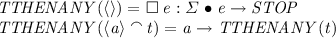
  If t is a trace of S, counterexamples to this refinement check provide traces , where e is not in the set initials(S/t). Thus, we obtain initials(S/t) by considering the events in $\varSigma$ for which no such counterexample exists.

Currently, our prototype calls FDR many times from scratch. As a future optimization, we will incorporate the caching of the internal results of the FDR, to speed up posterior invocations with the same model.

We have used our prototype to carry out two case studies, the Transputer-based sensor for autonomous vehicles in [23], and the Emergency Response System (ERS) in [2]. The sensor is part of an architecture where each sensor is associated with a Transputer for local processing and can be part of a network of sensors. The ERS allows members of the public to identify incidents requiring emergency response; it is a system of operationally independent systems (a Phone System, a Call Center, an Emergency Response Unit, and so on). The ERS ensures that every call is sent to the correct target. It is used in [18] to assess the deadlock detection of a prototype model checker for Circus.

For each case study, we have randomly generated 1000 finite SUTs with the same event alphabet. The experimental results confirm what we expected from the lemmas of the previous section. Namely, all incorrect SUTs are identified and the procedure terminates for all finite SUTs identified in Lemma 3. The prototype tool and the CSP model for the sensor, the ERS and other examples are in http://www.github.com/adenilso/CSP-FD-TGen. The data for the SUTs used in this case study is also available.

7 Conclusions

In this paper, we have investigated how fault domains can be used to guide test generation from CSP models. We have cast core notions of fault-domain testing in the context of the CSP testing theory. For testing for traces refinement, we have presented a procedure which, given a specification and a fault domain, it tests whether an SUT trace refines the fault domain. If the SUT is incorrect, the procedure selects a test that can reveal the fault. In the case of a correct SUT, we have stated conditions that guarantee that the procedure terminates.

There are specifications for which the procedure does not terminate. We postulate that for those specifications, there is no finite set of tests that is able to demonstrate the correctness of the SUT. Finiteness requires extra assumptions about the SUT. We plan to investigate this point further in future work.

The CSP testing theory also includes tests for conf, a conformance relation that deals with forbidden deadlocks; together, tests for conf and traces refinement can be used to establish failures refinement. Another interesting failures-based conformance relation for testing from CSP models takes into account the asymmetry of controllability of inputs and outputs in the interaction with the SUT [6]. It is worth investigating how fault domains can be used to generate finite test sets for these notions of conformance.

References

Alberto, A., Cavalcanti, A.L.C., Gaudel, M.-C., Simao, A.: Formal mutation testing for Circus. IST 81, 131–153 (2017)
Andrews, Z., et al.: Model-based development of fault tolerant systems of systems. In: SysCon, pp. 356–363, April 2013
Cavalcanti, A., Gaudel, M.-C.: Testing for refinement in CSP. In: Butler, M., Hinchey, M.G., Larrondo-Petrie, M.M. (eds.) ICFEM 2007. LNCS, vol. 4789, pp. 151–170. Springer, Heidelberg (2007). doi:10.1007/978-3-540-76650-6_10
Cavalcanti, A.L.C., Gaudel, M.-C.: Testing for refinement in Circus. Acta Informatica 48(2), 97–147 (2011)
Cavalcanti, A., Gaudel, M.-C.: Data flow coverage for Circus-based testing. In: Gnesi, S., Rensink, A. (eds.) FASE 2014. LNCS, vol. 8411, pp. 415–429. Springer, Heidelberg (2014). doi:10.1007/978-3-642-54804-8_29
Cavalcanti, A., Hierons, R.M.: Testing with inputs and outputs in CSP. In: Cortellessa, V., Varró, D. (eds.) FASE 2013. LNCS, vol. 7793, pp. 359–374. Springer, Heidelberg (2013). doi:10.1007/978-3-642-37057-1_26
Chow, T.S.: Testing software design modeled by finite-state machines. IEEE Trans. Softw. Eng. 4(3), 178–187 (1978)
El-Fakih, K.A., et al.: FSM-based testing from user defined faults adapted to incremental and mutation testing. Program. Comput. Softw. 38(4), 201–209 (2012)
Fujiwara, S., von Bochmann, G.: Testing non-deterministic state machines with fault coverage. In: FORTE, North-Holland, pp. 267–280 (1991)
Gibson-Robinson, T., Armstrong, P., Boulgakov, A., Roscoe, A.W.: FDR3 — a modern refinement checker for CSP. In: Ábrahám, E., Havelund, K. (eds.) TACAS 2014. LNCS, vol. 8413, pp. 187–201. Springer, Heidelberg (2014). doi:10.1007/978-3-642-54862-8_13
Hierons, R.M., Ural, H.: Optimizing the length of checking sequences. IEEE TC 55(5), 618–629 (2006)
Huang, W., Peleska, J.: Exhaustive model-based equivalence class testing. In: Yenigün, H., Yilmaz, C., Ulrich, A. (eds.) ICTSS 2013. LNCS, vol. 8254, pp. 49–64. Springer, Heidelberg (2013). doi:10.1007/978-3-642-41707-8_4
Koufareva, I., Petrenko, A., Yevtushenko, N.: Test generation driven by user-defined fault models. In: Csopaki, G., Dibuz, S., Tarnay, K. (eds.) Testing of Communicating Systems. ITIFIP, vol. 21, pp. 215–233. Springer, Boston (1999). doi:10.1007/978-0-387-35567-2_14
Luo, G., et al.: Test selection based on communicating nondeterministic finite-state machines using a generalized Wp-method. IEEE TSE 20(2), 149–162 (1994)
Milner, R.: A Calculus of Communicating Systems. LNCS, vol. 92. Springer, Heidelberg (1980). doi:10.1007/3-540-10235-3
Moraes, A., et al.: A family of test selection criteria for timed input-output symbolic transition system models. SCP 126, 52–72 (2016)
Morell, L.J.: A theory of fault-based testing. IEEE TSEg 16(8), 844–857 (1990)
Mota, A., Farias, A., Didier, A., Woodcock, J.: Rapid prototyping of a semantically well founded Circus model checker. In: Giannakopoulou, D., Salaün, G. (eds.) SEFM 2014. LNCS, vol. 8702, pp. 235–249. Springer, Cham (2014). doi:10.1007/978-3-319-10431-7_17
Nogueira, S., Sampaio, A.C.A., Mota, A.C.: Test generation from state based use case models. FACJ 26(3), 441–490 (2014)
Peleska, J.: Test automation for safety-critical systems: industrial application and future developments. In: Gaudel, M.-C., Woodcock, J. (eds.) FME 1996. LNCS, vol. 1051, pp. 39–59. Springer, Heidelberg (1996). doi:10.1007/3-540-60973-3_79
Petrenko, A., Yevtushenko, N.: Testing from partial deterministic FSM specifications. IEEE TC 54(9), 1154–1165 (2005)
Petrenko, A., et al.: On fault coverage of tests for finite state specifications. Comput. Netw. ISDN Syst. 29(1), 81–106 (1996)
Probert, P.J., Djian, D., Hu, H.: Transputer architectures for sensing in a robot controller: formal methods for design. Concurr. Pract. Exp. 3(4), 283–292 (1991)
Roscoe, A.W.: Understanding Concurrent Systems. Springer, London (2011). doi:10.1007/978-1-84882-258-0
Tretmans, J.: Test generation with inputs, outputs, and quiescence. In: Margaria, T., Steffen, B. (eds.) TACAS 1996. LNCS, vol. 1055, pp. 127–146. Springer, Heidelberg (1996). doi:10.1007/3-540-61042-1_42
Yu, Y.T., Lau, M.F.: Fault-based test suite prioritization for specification-based testing. Inf. Softw. Technol. 54(2), 179–202 (2012)
Acknowledgements
The authors would like to thank the partial financial support of the following entities: Royal Society (Grant: NI150186), FAPESP (Grant: 2013/07375-0). The authors also are thankful to Marie-Claude Gaudel, for the useful discussion in an early version of this paper.
Author information
Authors and Affiliations
Corresponding author
Editor information
Editors and Affiliations
Rights and permissions
Copyright information
© 2017 IFIP International Federation for Information Processing
About this paper
Cite this paper
Cavalcanti, A., Simao, A. (2017). Fault-Based Testing for Refinement in CSP. In: Yevtushenko, N., Cavalli, A., Yenigün, H. (eds) Testing Software and Systems. ICTSS 2017. Lecture Notes in Computer Science(), vol 10533. Springer, Cham. https://doi.org/10.1007/978-3-319-67549-7_2
Download citation
DOI: https://doi.org/10.1007/978-3-319-67549-7_2
Published:
Publisher Name: Springer, Cham
Print ISBN: 978-3-319-67548-0
Online ISBN: 978-3-319-67549-7
eBook Packages: Computer ScienceComputer Science (R0)