
Abstract
Automated characterization of online social behavior is becoming increasingly important as day-to-day human interaction migrates from expensive “real world” encounters to less expensive virtual interactions over computing networks. The effective automated characterization of human interaction in social media has important political, economic, social applications.
New analytic concepts are presented for the extraction and enhancement of salient numeric features from unstructured text. These concepts employ relatively simple syntactic metrics for characterizing and distinguishing human and automated social media posting behaviors. The concepts are domain agnostic, and are empirically demonstrated using posted text from a particular social medium (Twitter).
An innovation uses a feature-imputation regression method to perform feature sensitivity analysis.
You have full access to this open access chapter, Download conference paper PDF
Keywords
1 Background
The characterization of text threads in social media can be done using either or both of syntactic methods (e.g., “bag-of-words”), and semantic methods (e.g., Latent Semantic Indexing). Syntactic methods are much more mature and usually much less complex than semantic methods. For the purposes of this work, syntactic methods will refer to fundamentally distributional techniques that do not rely on semantic mapping. Syntactic methods will be those that do not require parsing, resolution of pronominal reference, geotagging, dictionary lookups, etc., but derive their results from term statistics.
Note: A “social medium” is defined here as any venue supporting public-access pseudo-anonymous self-initiated asynchronous data sharing.
2 The Venue: Twitter
The empirical demonstrations done during this research focuses on the characterization of user-generated content on Twitter, one of the simpler social media domains.
Twitter users submit (“post”) time-ordered sequences of text (called “tweets”, maximum of 140 text characters) through a simple text-window interface. These are made available to other Twitter users in several ways (e.g., “friending”, “following”).
The term thread refers to a time-ordered sequence of tweets posted by a particular user. Aggregation is facilitated by each user’s unique User Id number (a 1 to 17 digit positive integer) and a tweet time-stamp (epoch time). Tweets are not point-to-point communications; they generally function as personal status updates, but also frequently contain opinions about social issues, and items of general cultural interest (movies, sports, politics, world events, etc.) Twitter does not filter tweets for content (e.g., vulgarisms, hate speech).
The simplicity and lack of content constraints also makes Twitter an attractive venue for advertising, subscription services (e.g., weather/traffic reports, alerts), and other automated content. Tweets can contain any combination of free text, emoticons, chat-speak, hash tags, and URL’s. Because Tweets can contain URL’s, they can be malware vectors.
3 Types of Natural Language Text
Depending upon the type and amount of embedded structure used to present text, it is said to fall into two broad categories:
Structured text is text data that is organized into labeled units. The units are often referred to as “fields”. The labels are referred to as “metadata”, and give contextual information about the field (e.g., what data the field contains, its metric units and ranges, what the data “mean”, etc.)
Unstructured text is text data that is not organized into labeled units. In particular, unstructured text has relatively little embedded metadata. The content must provide its own context.
4 The Data Source
Twitter maintains a website for servicing data requests posted by those holding Twitter Developer credentials. Developers obtain these credentials through an online application process.
Credentialed developers may request information for Twitter user accounts by posting requests to the Twitter API (application program interface) at a URL (uniform resource locator) provided by Twitter. Requests can be made for specific accounts based upon their User Identification Numbers. Requests can also be made for random samples of accounts selected by Twitter. Requested data are returned as a hierarchical data structure called JSON (JavaScript Object Notation).
5 Data Form
Data for this work consist of the threads for 8,845 users, each having at least one tweet, and no more than 200 tweets. The users were randomly selected by Twitter from its international user base. Most, but not all, tweets used are in English.
6 Text Data Ground Truth Tagging
Tweet text for 101 user threads was evaluated manually by a team of English-speaking readers, all experienced users of social media. Because the intention is to model the perceptions of human content consumers, readers were instructed not to collaborate, and to use their personal intuition to decide which of the threads they reviewed were likely the result of human posting behaviors, and which were likely the result of automated posting (BOT’s). Ten readers participated, with each of the threads evaluated by at least 2 readers.
Sixty-five of the 101 threads were tagged as either “human generated” or “BOT generated” by majority vote of the readers of that thread. That experienced readers could not agree on the tagging of 36 out of 101 threads illustrates the difficulty of ground-truth assignment in this domain.
7 Extrapolation of Ground Truth Tags
The BOT-NotBOT tags from the 65 manually tagged threads were extrapolated to the larger corpus of 8,845 threads using a population-weighted N-Nearest Neighbor Classifier having the 65-thread set as the standard. N was allowed to vary from 1 to 20; the tagging for N = 5 was chosen for the extrapolation, because it best matched the class proportions of the 65-thread standard.
Following Hancock et al. [4], several angles-only metrics were used to project each feature vector into a low (nominally 4–8) dimensional Euclidean space for visualization and analysis.
8 The Content Data Elements and Their Encoding
The text constituting each of the 8,845 user threads was rolled up into a normalized 23-dimensional numeric feature vector quantifying certain low-level syntactic user posting behaviors the user (more complete description below).
Below are linguistic attributes that our team felt would be useful for discriminating automated posting behaviors from human posting behaviors. These attributes provide the rationale for the features that were encoded from the twitter text. The resulting features were used to generate mathematical “signatures” for online behaviors. In this way, they augment account-level demographic features (e.g., user time-zone, user language) to create a rich, high-fidelity information space for behavior mining and modeling.
-
1.
The relative size and diversity of the account vocabulary
Content generated by automated means tends to reuse complex terms, while naturally generated content has a more varied vocabulary, and terms reused are generally simpler.
-
2.
The word length mean and variance
Naturally generated content tends to use shorter but more varied language than automatically generated content.
-
3.
The presence/percentage of chatspeak
Casual, social users often employ simple, easy to generate graphical icons, called emoticons. Sophisticated non-social users tend to avoid these unsophisticated graphical icons.
-
4.
The presence and frequency of hashtags
Hash tags are essentially topic words. Several hash tags taken together amount to a tweet “gist”. A table of these could be used for automated topic/content identification and categorization.
-
5.
The number of misspelled words
It is assumed that sophisticated content generators, such as major retailers, will have a very low incidence of misspellings relative to casual users who are typing on a small device like a phone or tablet.
-
6.
The presence of vulgarity
Major retailers are assumed to be unlikely to embed vulgarity in their content.
-
7.
The use of hot-button words and phrases (“act now”, “enter to win”, etc.)
Marketing “code words” are regularly used to communicate complex ideas to potential customers in just a few words. Such phrases are useful precisely because they are hackneyed.
-
8.
The use of words rarely used by other accounts (e.g., Tf.Idf scores) [1]
Marketing campaigns often create words around their products. These created words occur nowhere else, and so will have high Tf.Idf scores.
-
9.
The presence of URLs
To make a direct sale through a tweet, the customer must be engaged and directed to a location where a sale can be made. This is most easily accomplished by supplying a URL. URL’s, even tiny URL’s, can be automatically followed to facilitate screen scraping for identification/characterization.
-
10.
The generation of redundant content (same tweets repeated multiple times)
It is costly and difficult to generate unique content for each of thousands of online recipients. Therefore, automated content (e.g., advertising) tends to have a relatively small number of stylized units of content that they use over and over.
A vector of text features is derived for each user. This is accomplished by deriving text features for each of the user’s tweets, then rolling them up. Therefore, one content feature vector is derived for each user from all of that user’s tweets, as follows:
-
1.
Collect the user’s most recent (up to 200) tweet strings into a single set (a thread).
-
2.
Convert the thread text to upper case for term matching.
-
3.
Scan the thread for the presence of emoticons, chat-speak, hash tags, URL’s, and vulgarisms, setting bits to indicate the presence/absence of each.
-
4.
Remove special characters from the thread to facilitate term matching
-
(a)
Create a frequency histograms for the thread. Vocabulary word from a twitter word list. The bins represent the 5,000 most frequently used Twitter words, arranged in order of decreasing Twitter frequency.
-
(a)
-
5.
Create a Redundancy Score for the Thread. This is done by computing and rolling up (sum and normalize) the pairwise similarities of the tweet strings within the thread using six metrics: Euclidean Distance, RMS-Distance, L1 Distance, L-Infinity Distance, Cosine Distance, and the norm-weighted average of the five distances.
-
6.
The thread text feature vector then contains as vector components the emoticon flag, the chat-speak flag, the hash tag flag, he URL flag, the vulgarity flag, the Redundancy score, and the selected term histogram (Fig. 1).
Fig. 1. 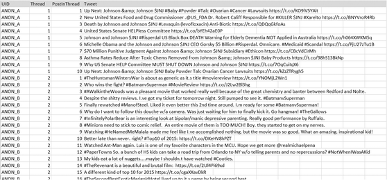
For the sake of definiteness and intuition building, the figure above shows actual tweet threads for two Twitter users.

9 Experiment 1: Feature Selection by Brute Force
Direct blind-evaluation of all 223 = 8,388,608 possible feature sets was performed to provide definitive feature evaluation.
When many columns of data are available, choosing the “right” ones to use is hard, for a number of reasons:
-
1.
Having many columns means many “dimensions” when viewed geometrically
-
2.
The data consist of columns that can interact in complicated ways. For example, two “weak” pieces of evidence together sometimes provide more information than one “strong” piece of evidence alone.
-
3.
There are a huge number of possible combinations in which columns could be chosen/rejected as features for a data mining project, so it is time-consuming to check them all. For example, if there are 20 columns, there are 220 − 1 > 1,000,000 ways to choose which subset of features to use.
The information assessment begins by reading in the data to be analyzed, and computing the means and standard deviations for each of the ground truth classes. That is, the means and standard deviations are computed for each column for all the rows that are in ground truth class 1, giving the “center” and “variability” of the class 1 data; then, for class 2 rows, and so on.
To determine which columns contain information useful for classification of the data into its ground truth classes, all possible subsets of the available columns are tested; the subsets giving the best results with a weighted nearest-neighbor classifier are cataloged. The process proceeds as follows:
-
Step 1: Read in the data file containing the numericized feature data
-
Step 2: Segment the data file in calibration, training and validation files
-
Step 3: Compute the centroids, feature standard deviations calibration data
-
Step 4: Select a subset of the columns to test (a “clique”)
-
Step 5: Use the centers and standard deviations computed in Phase A for the clique to assign each data point in the training segment to a class as depicted in Fig. 2.
Fig. 2. 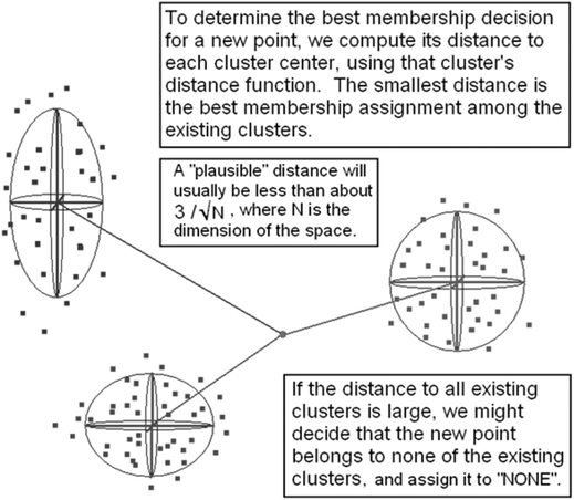
Classification by nearest class centroid

Repeat steps 4 and 5 for all possible feature cliques. With 23 features, this is 223 = 8,388,608 unique feature representations of the data. The features in the “best” clique (had the highest accuracy score on the test set) are the ones that, as a group, have the most useful information for classification of those tested. This “winning team” comprises our selected feature set.
To create a numeric measure of the classification power of a subset of the available features, this very fast weighted nearest-neighbor classifier is run repeatedly on a calibration set with various sets of features, and the best collection is remembered. Also, if the same feature appears in many high-performing feature sets, it is reasonable to conclude that it is probably “good”. In this way, the clustering algorithm described here is used to “game” feature sets in a “Monte Carlo” fashion.
The spreadsheet below shows the classification power of various feature sets. In the table below, “1” means that columns feature was present in that set, while “0” means it was not. In this experiment, only the 2,500 highest blind-accuracy feature sets were cataloged. This output gives the performance measures for all of them so the user can see the value of including/excluding the various feature combinations (Fig. 3).

Feature sets and their effectiveness
Each feature clique is a row; a “0” means that feature was not used in that clique, excluded, and a “1” means that feature was used in that clique. Performance for each clique is in columns 2 and 3. The bottom row shows the proportion of the top 2,500 cliques that used the feature in the corresponding column. For example, the feature indicating the use of adjectives was used in 72.7% of the 2,500 best feature sets. This provides a relative ranking of features with respect to how they contribute in context.
10 Experiment 2: Sensitivity Testing by Feature Imputation
An “intra/inter-vector” feature imputation scheme is now described that uses a reference data set to determine the most likely fill values for the features of a feature vector (this is called “feature imputation”). For example, if a vector has all features present except one, the existing features and the reference set are used to make a best estimate of the missing feature. This is equivalent to asking, “What feature value should be placed here, given the values of the other features in the vector?”
The imputation software ingests a feature vector file, and infers, in this way, a new value for *every* feature of *every* vector in the whole file, using patterns from a reference feature vector file as the standard.
11 The Imputation Algorithm
A simple inter-vector imputation method just replaces missing values with their population means, a O(n) process. This naïve approach is simple, but ignores feature context within the vector. For numeric data, a more sophisticated method is the nearest neighbor normalization technique. This can be applied efficiently even to large data sets having many dimensions (in a brute force approach this is a O(n2) process). This technique proceeds in the following manner for each missing feature in a given vector, V1:
-
1.
From the reference set of feature vectors, find the one, V2, which:
-
(a)
Shares a sufficient number of populated fields with the vector to be imputed (this is to increase the likelihood that the nearest vector is representative of the vector being processed).
-
(b)
Has a value for the missing feature, Fm.
-
(c)
Is nearest the vector to be imputed (possibly weighted).
-
(a)
-
2.
Compute the weighted norms of the vector being imputed, V1, and the matching vector found in step 1, V2, in just those features present in both.
-
3.
Form the normalization ratio Rn = |V1|/|V2|.
-
4.
Create a preliminary fill value P = Rn * Fm.
-
5.
Apply a clipping (or other) consistency test to P to obtain F’m, the final, sanity checked fill value.
-
6.
Fill the gap in V1 with the value F’m.
This method was used to perform a feature sensitivity analysis with respect to the ground truth in the following way:
The 8,845 thread set described above was divided into two sets by inferred ground truth: Those tagged as BOT were placed in one file, and those tagged as non_BOTS in another.
The 8,845 thread set was divided into two sets by inferred ground truth: Those tagged as BOT were placed in one file, and those tagged as non_BOTS in another.
The imputation scheme was then used to impute the non-BOT feature vectors using the BOT file as the reference set. Comparing the before and after imputation versions of the non-BOT file addresses Question A:
“Which features must be altered, in what ways, by how much, to make a non-BOT resemble a BOT?”
This process was repeated, this time using the Intra/Inter-Vector Regression scheme to impute the BOT feature vectors using the non-BOT file as the reference set. Comparing the before and after imputation versions of the BOT file addresses Question B:
“Which features must be altered, in what ways, and by how much, to make a BOT resemble a non-BOT?”
These are important and interesting questions that, among other things, provide objective insight into how BOT-characterization is seen in each feature. They also provide insight into how to disguise a BOT as a non-BOT. It is interesting to note that the changes required to make a BOT look like a non-BOT are the reverse of the changes required to make a non-BOT look like a BOT (Figs. 4 and 5).

The figure immediately above shows the “before” and “after” feature means for BOT data imputed from Non-BOT data. The light colored line is the z-weighted delta between the “before” and “after” representations.

The “before” and “after” feature means for the non-BOT data imputed from the BOT data. The light colored line is the z-weighted delta between “before” and “after” featuress.
The following is a tabulation of some “before imputation” and “after imputation” statistics for each of the 23 features. The first two columns give the feature number and name, respectively. Columns 3 and 4 are the feature means of the BOT data before and after imputation from the non-BOT data. Column 5 is column 4 minus column 3 (the change in the means due to imputation). Columns 6 and 7 are the feature standard deviations of the BOT data before and after imputation from the non-BOT data. Column 8 is column 7 minus column 6 (the change in the standard deviations due to imputation) (Fig. 6).

Before and after imputation statistics
Columns 9 and 10 are the feature means of the non-BOT data before and after imputation from the BOT data. Column 11 is column 10 minus column 9 (the change in the means due to imputation). Columns 12 and 13 are the feature standard deviations of the non-BOT data before and after imputation from the BOT data. Column 14 is column 13 minus column 12 (the change in the standard deviations due to imputation).
Notice that imputation from non-BOTs to BOTS moves the means in the direction opposite the direction of imputation from BOTs to non-BOTs, as would be expected.
To verify the effectiveness of imputation in “nudging” vectors from one class to another, a classifier that discriminates between BOT and non-BOT data is applied to the imputed data. If the imputation has been effective, the post-imputation BOTS will be classified as non-BOTs, and the post imputation non-BOTs will be classified as BOTS.
In fact, when the imputed data is classified by the original data using a nearest neighbor classifier, the ground truth tags are reversed for 100% of the vectors, as expected.
12 Future Work
This work describes a characterization method for content data. Future work will leverage the factor analysis it provides, which previous work has shown [1] can be used to determine which members of a forum are least committed to their clique, and exactly what would be required to move them out of their current clique. This is a type of “cultural terrain-forming”.
These observations suggest that opportunities for objective, quantitative proactive social media psy-ops planning could use the imputation sensitivities to estimate the following:
-
1.
How each feature’s effect on BOT-non-BOT assignment is quantified
-
2.
How to optimally impersonate a member
-
3.
How to identify imposters/impersonators (psycho-anomaly detection)
-
4.
Deriving posts that would tend to foment or mitigate conflict among cliques.
References
Hancock, M., et al.: Modeling of social media behaviors using only account metadata. In: 8th International Conference on Applied Human Factors and Ergonomics, Orlando, Florida, July 2016
Hancock, M., et al: Multi-cultural empirical study of password strength vs. ergonomic utility. In: 18th International Conference on Human Computer Interaction, Toronto, Canada, July 2016
Hancock, M., et al.: Field-theoretic modeling method for emotional context in social media: theory and case study. In: Schmorrow, D.D., Fidopiastis, C.M. (eds.) AC 2015. LNCS (LNAI), vol. 9183, pp. 418–425. Springer, Cham (2015). doi:10.1007/978-3-319-20816-9_40
Hancock, M., Sessions, C., Lo, C., Rajwani, S., Kresses, E., Bleasdale, C., Strohschein, D.: Stability of a type of cross-cultural emotion modeling in social media. In: Schmorrow, D.D., Fidopiastis, C.M. (eds.) AC 2015. LNCS (LNAI), vol. 9183, pp. 410–417. Springer, Cham (2015). doi:10.1007/978-3-319-20816-9_39
Hancock, M.: Novel methods for adjudicating multiple cognitive decision models. In: 2nd International Augmented Cognition Conference, San Francisco, CA, October 2006
Hancock, M., Day, J.: Exploring human cognition by spectral decomposition of a Markov random field. In: 1st International Augmented Cognition Conference, Las Vegas, NV, July 2005
Hancock, M.: A cognitive engineering methodology for building multi-level fusion applications. In: Northrop Grumman Data Fusion Conference, Aurora, CO, November 2007
Hancock, M.: Automating the characterization of social media culture, social context, and mood. In: Science of Multi-Intelligence Conference (SOMI), Chantilly, VA (2014)
Hancock, M.: Data mining: technology and practice in the real world. In: Tutorial Notes of the SIAM International Data Mining Conference (SDM 2003) (2003)
Author information
Authors and Affiliations
Corresponding author
Editor information
Editors and Affiliations
Rights and permissions
Copyright information
© 2017 Springer International Publishing AG
About this paper
Cite this paper
Hancock, M. et al. (2017). Some Syntax-Only Text Feature Extraction and Analysis Methods for Social Media Data. In: Schmorrow, D., Fidopiastis, C. (eds) Augmented Cognition. Neurocognition and Machine Learning. AC 2017. Lecture Notes in Computer Science(), vol 10284. Springer, Cham. https://doi.org/10.1007/978-3-319-58628-1_37
Download citation
DOI: https://doi.org/10.1007/978-3-319-58628-1_37
Published:
Publisher Name: Springer, Cham
Print ISBN: 978-3-319-58627-4
Online ISBN: 978-3-319-58628-1
eBook Packages: Computer ScienceComputer Science (R0)