
Abstract
Collaborative manufacturing chains (CMSs) are understood as networks of manufacturing units that are highly specialized, cooperation-independent and economically autonomous. CMSs are becoming ever more complex in today’s global market and one pertinent task for supply chain designers/managers is to handle outsourcing decision-making problems, by which such complexity can be reduced. In this paper, we propose to solve this problem through generation of alternative collaborative manufacturing chains that are benchmarked using topological complexity metrics. For this purpose, firstly supply chain structures are modelled. Subsequently, topological complexity measures for each possible configuration network are quantified. Finally, optimal supply chain configurations are selected.
You have full access to this open access chapter, Download conference paper PDF
Keywords
1 Introduction
One of the main challenges for original equipment manufacturers (OEMs) is transformation of their business strategies into mass customization (MC). This trend is pulled by the growing demand for tailor-made mass produced products and pushed by rapid development of modern supporting technologies such as information technologies, additive manufacturing, 5th generation mobile networks, identification technologies and others. Companies aligned with this strategy will need to adopt collaborative manufacturing network models. As it is known, this leads to an increase in manufacturing complexity. Therefore, companies with higher degree of customization might focus on reducing the complexity of the production processes, since complexity problems not only affect the production processes, but also managerial processes [1, 2]. Although this objective is quite clear, the way to achieve it is not. Then, the following research questions can be stated. RQ 1 : Can suitable alternative supply chain (SC) structure(s) be modelled? RQ 2 : If yes, how to identify the least complex structure?
An identification of complexity metrics is the first precondition for solving such problem. Prior to this task, it would be helpful to have a basic understanding of what factors affect the manufacturing complexity. Typical feature for MC is that products consist from several modules and each module can have a certain number of variants. Combinations of these variants contribute to high product variety that triggers high manufacturing complexity [3]. The supply chain creates a network of interconnected producers. At each producer, selected components according to customer needs are assembled onto the partially finished product. Finally, end product is finalized at the OEM. The goal of paper is to propose a framework for modelling of alternative collaborative supply chain (CSC) structures and to provide a description of possible complexity mitigation in collaborative manufacturing chains.
2 Generating Alternatives to Collaborative Manufacturing Structures
Generating the alternatives of CSC structures is useful especially when obtained structures can be utilized for practical guidance, and applied in conjunction with a selection of optimal collaborative manufacturing models. Moreover, it helps layout designers, among others, to increase productivity and to reduce costs and complexity. Especially, the network complexity reduction is recently in the centre of managers’ attention as assembly SC systems are becoming increasingly complex. On the other hand, high flexibility of supply chains is required to obtain short delivery times.
Commonly for this purpose, graph theory is applied. Assembly SCs can be represented by tree directed graphs, in which each node in the chain has at most one successor, but may have any number of predecessors. Convergent SCs are divided into two basic types: modular and non-modular. In the modular structure, the intermediate sub-assemblers are understood as assembly modules while the non-modular structure consists of only original suppliers and a final assembler (root node). Steps to identify optimal assembly SC structures have been clearly specified by Zhu et al. [4] in the following steps:
-
(a) Generation of all possible SC structures;
-
(b) Quantification of topological complexity values for each possible configuration;
-
(c) Selection of the optimal SC configurations.
The same authors outlined the way forward to model possible SC structures depending on the number of original suppliers i. If a SC has from two to four original suppliers, then we obtain one, two, five different assembly SCs. In the case of five suppliers i = 5, 12 different assembly SC networks can be generated, as can be seen in Fig. 1 (Class #5).

All possible SC networks for five original suppliers (Class #5) [5].
Analogically, it is possible to generate topological structures of assembly SC networks for any number of original suppliers, starting from i ≤ 2–∞). From here on, assembly SC structures are further considered are CSC structures.
3 Complexity Mitigation in CSC Structures
In the previous Sect. 2, SCs have been modelled by unlabeled graphs. However, CSCs correspond with labelled graphs. Therefore, in order to mitigate complexity of CSC structures, it is advisable to follow these steps:
-
1.
Firstly, to transform a realistic SC system into a labelled graph and subsequently to assign a corresponding SC structure to that graph. A simple example is shown in Fig. 2.
Fig. 2. 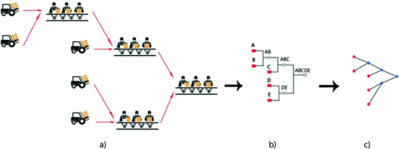
(a) CSC realistic layout; (b) transformation into a labelled graph; (c) transformation into the SC network No. 10 in Class #5.
-
2.
Identify alternative SC structures to the corresponding SC considered as the original one. Such alternative structures are available in all lower classes “i” of the SC structures than the class of the given assembly SC structure. As an example, original SC structure from Fig. 2(c) can be used.

Then, all alternative CSC networks can be identified as depicted in Fig. 3 below. Such alternative CSC structures are empirically less complex and at the same time they keep the predefined assembly sequence unchanged. From the graph theory viewpoint, obtained alternative graphs in the lower topological classes are then homeomorphic to the original labelled graph. From a practical point of view, such alternatives of CSC systems can be achieved based on outsourcing method that often allows company’s clients to reach better, faster, and more sustainable results.

Original CSC structure with i = 5 and related alternative SC networks
-
3.
Finally, substitute intuitive methods for complexity comparison of benchmarked CSC structures by appropriate and effective indicators of topological complexity.
Coming back to Fig. 3, four alternative CSC structures are taken from SC topological Classes of #4, #3 and #2. Then, when considering, e.g. the CSC structure taken from the topological Class #4 (namely, graph No. 5), it is assumed that node DE with two external suppliers is substituted by one external supplier of the DE module. It is also evident that in alternative CSC models, the predefined sequences are unchanged. Arrangements of other two alternative CSC structures (graphs No. 4, No. 2, and No. 1) are analogical. In the next step, it is useful to benchmark the complexity of original CSC structure (graph No. 10) against the four alternative CSC networks. For this purpose, in the next section two alternative complexity indicators are described.
4 Approaches to Structural Complexity of CSC
Metrics of structural complexity for specific or general networks can help companies not only design SC structures but also to better understand their topological properties. Layout design complexity metrics can be effectively used especially when comparing two or more CSC structures. Several studies in the literature, e.g. [6–15] can be found dealing with complexity indicators for structural complexity measurement of manufacturing and logistics systems.
Since there are several types of assembly supply chain models, not all the complexity indicators are equally effective for different groups of networks. Based on the literature review aimed at current developments in assessment of SC complexity, the following gap has been identified: So far, there is no SC framework that identifies structural relationship among the system vertices.
Respecting this fact, two complexity indicators are proposed to satisfy the need for effective SC complexity assessment.
4.1 Vertex Degree Index I vd
According to Shannon’s information theory [16], the entropy of information H(α) in describing a message of N system elements, distributed according to some equivalence criterion α into k groups of N 1 , N 2 ,…, N k elements, is calculated by the formula:
where p i specifies the probability of occurrence of the elements of the i th group.
Since it is of interest to characterize entropy of information of a network according to [16], it is possible to substitute symbols or system elements for the vertices.
In order to define the probability for a randomly chosen system element i it is possible to formulate general weight function as p i = w i /Σwi, assuming that Σp i = 1. Considering the system elements, the vertices, and supposing the weights assigned to each vertex to be the corresponding vertex degrees, one easily distinguishes the null complexity of the totally disconnected graph from the high complexity of the complete graph. Shannon defines information as:
where H max is maximum entropy that can exist in a system with the same number of elements.
Subsequently, the information entropy of a graph with a total weight W and vertex weights w i can be expressed in the form of the equation:
where the total number of vertices within a SC is V. Since the maximum entropy is when all w i = 1, then
By substituting \( W = \sum\nolimits_{i = 1}^{V} {{ \deg }(v)_{i} } \) and w i = deg(v) i , the information content of the vertex degree distribution of a network called as Vertex degree index (I vd ) is derived by Bonchev and Buck [17] that is expressed as follows:
An explanation of the deg(v) i and I vd calculations are depicted in Fig. 4.

Information content I vd of the case SC structure with i = 6
Following the procedure obtaining I vd information content, Table 1 summarizes values of I vd indicator for all CSC structures in Classes #2–5, while suitable alternative CSC structures are highlighted.
4.2 Axiomatic Design-Based Complexity - Systems Design Complexity (SDC)
The main definition of Axiomatic design [18] states that any process can be seen in four main domains: process, functional, customer and physical. The process consists of several steps and at the end results with structured relations between customer needs, functional requirement (FR) and selected design parameters (DP). These relations or dependencies between FRs and DPs within any design hierarchy can be expressed by the relation: FR = [A] DP. This relation can be expressed as each FR on the product component depends on the specific design parameter (DP) of the product specified by customer, so that each such dependency [A] can be understood as existing relation of FR on DP. If in the design matrix of any process element A refers to “0”, then FR is not in relation with DP. And vice versa for “1”, where there is relation between the DP and FR.
According to the SDC approach, we indicate each initial node of the CSC model as a FR (for example FR 1 to FR 10 at Class #10) and each sub-assembly vertex as DP (for example DP 1 to DP 3 depending on the specific CSC structure shown in Fig. 5. This is because initial nodes practically represent company requirements on suppliers and specify the number of initial nodes into CSC. This way, the transformation of all repeated CSC is possible and valuable. Analogically, we can transform each CSC structure into an axiomatic design matrix. For such matrices it is characteristic that individual elements [A] are mostly non-zero and thus the FRs cannot be satisfied independently.

CSC structure with 10 FRs and 3 DPs transformed into a design matrix.
We propose the following SDC measure (in nats) based on the Axiomatic Design (AD) expressed as follows:
where the volume is equal to unity and ‘Nj’ is interpreted as number of direct relations per single DP of the design matrix. Case transformation of the design matrix into a coupled design including calculation of SDC complexity is depicted in Fig. 5.
Subsequently, the following Table 2 summarizes the values of SDC for all CSC structures, while suitable alternative structures and their SDC complexity values are highlighted.
5 Comparison of the Approaches to Structural Complexity
The above presented indicators can be assessed in the view of their applicability:
In the case of I vd indicator and its application, 12 graphs in the same SC Class #5 can be divided into six levels of structural complexity (see Table 1). The mentioned complexity indicator is therefore not an optimal measure of structural complexity of CSCs.
On the other hand, AD-based indicator SDC considers graphs links as interactions between nodes. Then, complexity values of SDC indicator for the same CSC structures in Classes from #2 to #5 differ for each of the graphs (see Table 2).
Concluding the computational analysis using three structural complexity indicators, we may state that AD-based complexity suits best for the given purpose.
6 Conclusions
Complexity topology analysis of the CSC structures in this paper revealed potential tools to optimize any SC structures to be used in mass customization environment. Moreover, it has been found that modelling of all possible SC is purposeful because any existing structure can be simplified using the approach presented above to obtain less complex SC alternative(s). Secondly, the two complexity metrics, namely I vd and SDC to capture structural properties of all possible CSC networks have been benchmarked. The SDC indicator fits best for the decision-making about the optimal collaborative chain as it considers also links between nodes and their interoperability.
Subsequently it was shown that the proposed approach to model CSC networks can be effectively used in MC manufacturing environment. Finally, a draft concept to product variety quantification has been outlined as a precondition for posterior solutions of product variety complexity mitigation.
References
Stump, B., Badurdeen, F.: Integrating lean and other strategies for mass customization manufacturing: a case study. J. Intell. Manuf. 23(1), 109–124 (2012)
Brosch, M., Beckmann, G., Krause, D.: Approach to visualize the supply chain complexity induced by product variety. In: Proceedings of 18th International Conference on Engineering Design (ICED 2011), Impacting Society through Engineering Design, p. 10. TU Denmark, Copenhagen (2011)
Blecker, T., Friedrich, G., Kaluza, B., Abdelkafi, N., Kreutler, G.: Information and Management Systems for Product Customization, vol. 7. Springer Science & Business Media, New York (2004)
Zhu, X., Hu, S.J., Koren, Y., Marin, S.P.: Modeling of manufacturing complexity in mixed-model assembly lines. J. Manuf. Sci. E-T ASME 130(5), 1–10 (2008)
Modrak, V., Marton, D., Bednar, S.: Modeling and determining product variety for mass-customized manufacturing. Procedia CIRP 23, 258–263 (2014)
ElMaraghy, H., AlGeddawy, T., Samy, S.N., Espinoza, V.: A model for assessing the layout structural complexity of manufacturing systems. J. Manuf. Syst. 33(1), 51–64 (2014)
Crippa, R., Bertacci, N., Larghi, L.: Representing and measuring flow complexity in the extended enterprise: the D4G approach. In: Congress For Research in Logistics (2006)
Modrak, V., Bednar, S., Marton, D.: Generating product variations in terms of mass customization. In: 2015 IEEE 13th International Symposium Applied Machine Intelligence and Informatics (SAMI). IEEE (2015)
Wang, H., Zhu, X., Hu, S.J., Koren, Y.: Complexity analysis of assembly supply chain configurations. In: ASME 9th Biennial Conference on Engineering Systems Design and Analysis, pp. 501–510. American Society of Mechanical Engineers, Michigan (2008)
Koren, Y., Heisel, U., Jovane, F., Moriwaki, T., Pritschow, G., Ulsoy, G., Van Brussel, H.: Reconfigurable manufacturing systems. CIRP Ann. Manuf. Technol. 48(2), 527–540 (1999)
Wang, H.: Product variety induced complexity and its impact on mixed-model assembly systems and supply chains. Doctoral dissertation, General Motors (2010)
Frizelle, G.: Measuring complexity as an aid to developing operational strategy. Int. J. Oper. Prod. Manag. 15(5), 26–39 (1995)
Deshmukh, A.V., Talavage, J.J., Barash, M.M.: Complexity in manufacturing systems, Part 1: analysis of static complexity. IIE Trans. 30(7), 645–655 (1998)
Espinoza Vega, V.B.: Structural complexity of manufacturing systems layout. M.Sc. thesis, University of Windsor, Canada (2012)
Németh, P., Foldesi, P.: Efficient control of logistic processes using multi-criteria performance measurement. Acta Technica Jaurinensis 2, 353–360 (2009)
Shannon, C.E.: A mathematical theory of communication. Bell Syst. Tech. J. 27, 379–423 (1948)
Bonchev, D., Buck, G.A.: Quantitative measures of network complexity. In: Bonchev, D., Rouvray, D.H. (eds.) Complexity in Chemistry, Biology and Ecology, vol. 1, pp. 191–235. Springer, Heidelberg (2005)
Suh, N.P.: Complexity in engineering. CIRP Ann. Manuf. Technol. 54(2), 46–63 (2005)
Author information
Authors and Affiliations
Corresponding author
Editor information
Editors and Affiliations
Rights and permissions
Copyright information
© 2016 IFIP International Federation for Information Processing
About this paper
Cite this paper
Modrak, V., Bednar, S. (2016). Complexity Mitigation in Collaborative Manufacturing Chains. In: Afsarmanesh, H., Camarinha-Matos, L., Lucas Soares, A. (eds) Collaboration in a Hyperconnected World. PRO-VE 2016. IFIP Advances in Information and Communication Technology, vol 480. Springer, Cham. https://doi.org/10.1007/978-3-319-45390-3_35
Download citation
DOI: https://doi.org/10.1007/978-3-319-45390-3_35
Published:
Publisher Name: Springer, Cham
Print ISBN: 978-3-319-45389-7
Online ISBN: 978-3-319-45390-3
eBook Packages: Computer ScienceComputer Science (R0)