
Abstract
In order to support energy efficiency improvement, it is essential to monitor the energy performance and to make benchmarking with similar process or related Best Available Techniques. Among different key performance indicators that compare similar processes, the most relevant for the industrial sector is the specific energy consumption (SEC). With regard to the energy demand in an industrial process, a variable and fixed portion can generally be distinguished: as a direct consequence the amount of energy used per unit of product (SEC) usually decreases while the production rate increases. It should be noted that often production processes face variable demand over their utilization. Aim of this work is to propose a novel decision model to support the identification of the more suitable investment in energy efficiency given the variable demand expected, explicitly considering that the effect of investments in energy efficiency can be categorized in two main categories: those shifting the SEC curve and those flattening the SEC curve.
You have full access to this open access chapter, Download conference paper PDF
Keywords
1 Introduction
Energy efficiency is an essential part of a sustainable energy future as it helps reducing the energy consumption. In addition, energy efficiency leads to many other benefits, such as: it drives economic growth creating jobs and investment opportunities, it reduces greenhouse-gas emissions and air pollutants, it lowers fuel expenditures and it enhances energy security [1]. As it is shown in Fig. 1, the industrial sector is the greater energy consumer than any other end-use sectors, currently consuming about 50 % of the world’s total delivered energy [2, 3]. Moreover, in Fig. 2 it is possible to observe that, over the next 20 years, the worldwide industrial energy consumption is expected to grow from 3,900 Mtoe in 2014 to 5,000 Mtoe in 2035 by an average of about 6 % per year [4].

World shares of total energy use by end-use sector, 2011 [2]

Industrial sector energy consumption from 1990 to 2035 (Mtoe) [4]
Recently, energy efficiency in the industrial sector has emerged as one of the most significant manufacturing decision option and it is gaining an increasingly relevance [5, 6]. The key drivers for a gradual process of rethinking towards a more energy-efficient acting are: the energy turnaround in Europe including the “20-20-20” targets, the great impact of energy issue on the strategic objectives of industrial companies, which are costs, time and quality and, finally, the customers’ increasing ecological awareness [7–9]. However, industry often views energy as an operational cost instead of a competitive advantage: energy savings are perceived as incidental benefits of other actions rather than as a central value-generating proposition.
In order to reach higher levels of energy efficiency, it is important to monitor the progress of the energy performance of the company and to make comparisons with the performances of other firms (benchmarking). For that reason, key energy performance indicators (KPIs) have been introduced, such as the Specific Energy Consumption (SEC): i.e. the ratio between the total energy consumption and the physical/economic output value. Some of the advantages of this indicator are that it is not influenced by price fluctuations and can be directly related to process operations and technology choice. However, a comparison of energy use in different units and aggregate efficiency is effectively impossible without the conversion of the physical units’ value into a common economic value [10].
Generally, the energy consumption profile of an industrial plant is given by two contributions: one is fixed, given the production plant, and the other is variable depending on the production rate. Thus, the amount of energy consumed per unit of product, and so the value of the specific energy consumption, decreases with the increase of the production rate, as the incidence of the fixed share decreases (Fig. 3). In many cases, industrial plants have to face variable, uncertain and discontinuous demands, e.g. days with high production and days with no production, working times alternate with idle times. For that reason, a wide range of production rate interests the production and the required flexibility results in reduced energy efficiency and increasing costs [11]. Even the specific energy consumption is subject to uncertainty, as it is a function of the production rate. Consequently, investments in energy efficiency can be divided in two subcategories: investments that reduce the specific energy consumption equally for all the production (“SEC vertical shifting”) and investments that reduce the specific energy consumption differently for different production rate, i.e. flattening the curve of energy consumption (“SEC flattening”). See Fig. 3.

Effects on the specific energy consumption of different energy efficient investment
The approach followed to evaluate the investments is the NPV (Net Present Value) method, in addition to the easier Payback period (PB), because, even if it is quite complex to apply, it gives better results and it allows comparing investments with different characteristics [8, 12]. This work analyses the most suitable investment in energy efficiency for a given industrial plant under constant and uncertain demand profile. The remainder of the paper is organized as follows: Sect. 2 introduces the notations and assumptions, Sect. 3 presents the mathematical models of the different scenarios considered, Sect. 4 provides numerical examples to illustrate the proposed models and, finally, Sect. 5 concludes the paper summarizing main findings and providing suggestions for future research.
2 Assumptions and Notations
This paper considers the problem of identifying the most suitable investment in energy efficiency for a given industrial plant and a given demand profile.
The notation of the model is:
D | Annual demand rate [unit] |
P | Real production rate [unit/year] |
Pmax | Nominal production rate [unit/year] |
n | Investment’s lifespan [years] |
a0 | Initial sensitivity coefficient on the constant of the SEC’s curve |
b0 | Initial sensitivity coefficient on the slope of the SEC’s curve |
a | Sensitivity coefficient on the constant of the SEC’s curve |
b | Sensitivity coefficient on the slope of the SEC’s curve |
amin | Minimum value of the coefficient a |
bmax | Maximum value of the coefficient b |
c0,en | Energy cost per unit of production before investment [€/unit] |
cen | Energy cost per unit of production after investment [€/unit] |
pe | Energy price per kWh [€/kWh] |
SEC0 | Specific energy consumption before investment [kWh/unit] |
SEC | Specific energy consumption after investment [kWh/unit] |
S | Savings introduced with investments [€] |
ρ | Discount rate |
δa,shift | Decrease coefficient in the constant of the SEC per € increase in Ishift |
δa,flat | Decrease coefficient in the constant of the SEC per € increase in Iflat |
δb,flat | Decrease coefficient in the slope of the SEC per € increase in Iflat |
Ishift | Investment made to shift the SEC (decision variable) [€] |
Iflat | Investment made to flat the SEC (decision variable) [€] |
The main assumptions of the model are the following:
-
The demand rate D i is constant in Scenario 1, while in Scenario 2 it is uncertain and modelled with a stochastic distribution with parameters (α, β).
-
The nominal production rate is P max but the working one P is lower. Thus, due to the underuse, the performance of the plant is lower than the nominal one and inefficiencies are introduced.
-
The effective production rate corresponds to the demand rate (L4L assumption).
-
The SEC is usually represented by a power function of the production rate P. However, for simplicity, it has been considered an interval of production rate in which it is possible to approximate the SEC with a linear function (Fig. 4) of P, as following:
$$ SEC = a - b \cdot P $$(1)Fig. 4. 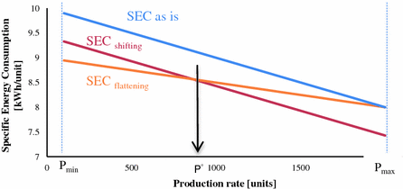
Specific energy consumption function with respect to the production rate
-
The energy price per kWh p e [€/kWh] is assumed to be constant.
-
The investment in vertical shifting, I shift , has effect on the constant of the curve, a. While the investment in flattening, I flat , has effect both on the constant, a, and on the slope, b, of the SEC’s curve.
-
Considering the diminishing marginal contribution of investments [13–15], a logarithmic investment function of the following form is used to describe the effect of the investments on the parameters of the specific energy consumption:
$$ x = x_{0} - \delta_{x} \cdot \ln \left( {I_{x} } \right) $$(2)where x identifies the SEC’s parameter affected by the investment (i.e. a or b).

3 Model’s Formulation
In the present work, it is considered a firm that has to select the amount of investment in vertical shifting or in flattening the specific energy consumption curve maximizing the NPV. Often the demand is uncertain, random and fluctuating; for that reason, the company has to face a wide interval of possible production rate. In this case, investment in flattening the specific energy consumption acquires greater relevance. Traditional capital budgeting investment decisions identify a profitable energy efficiency investment when the discounted sum of savings, S, is greater than the total investment cost, I. This net present value (NPV) provides an estimate of the net financial benefit provided to the organization if this investment is undertaken [12].
where
Savings, S i , are introduced by the reduction of the specific energy consumption and thus by the reduction of the energy cost of the production (Eq. 3). The subscript i identifies the year considered and it varies from 1 to n, which is the lifetime of the investment. In a first step, it has been considered the scenario where demand rate is constant (Scenario 1) evaluating the optimal investment decision for a given input value of the production rate. Then, in a second step, it has been modelled the demand rate and, thus, the production rate with a probability distribution (Scenario 2), defined in the assumption. Table 1 summarizes the demand modelling and the investment decisions of each considered scenario:
3.1 Scenario 1.1
In Scenario 1.1, the demand is constant and the only investment considered is the vertical shifting of the specific energy consumption (I shift ). It is possible to study the function and its derivatives in order to evaluate the convexity of the NPV function in I shift and to find the optimal value of \( {I_{shift}}^* \), that is:
3.2 Scenario 1.2
In Scenario 1.2, the demand is still constant as the previous scenario; however, the only investment considered is the flattening of the specific energy consumption (I flat ) and the optimal value of \( {I_{shift}}^* \) is:
4 Numerical Study
In the present section two examples are presented: in the first, general investment alternatives which impact the entire production plant are considered; while, in the second, the subject of the study is related to a particular sub-system. Example 1 illustrates the results of the models in a specific sector and compares the behaviour of the different scenarios. The parameters used in Scenario 1 are the following: D = 1500 units/year, Pmax = 2000 units/year, n = 10 year, ρ = 4 %, pe = 0.25 €/kWh, a0 = 10, b0 = 0.001, δa,shift = 0.04, δa,flat = 0.2, δb,flat = 0.0001. After a first insight in Scenario 1, in Scenario 2 we assumed that the demand is modelled with a uniform distribution with parameters (750, 1750); while the other parameters are the same. The numerical example, for a given production rate (Scenario 1) and for the uniform distribution (Scenario 2), leads to the following results (Table 2):
As can be observed in Table 2, both the investments result convenient (NPV > 0) and generates energy cost savings. In particular, Scenario 1.2 (i.e. the scenario in which the investment in flattening is considered) leads to a better result reducing the specific energy consumption of about 3 % with respect to the as – is scenario, i.e. without any kind of investment, in which the SEC was 8.5 kWh/unit, and leading to a NPV greater than the one with investment in vertical shifting; while the payback period is almost equal. An interesting value of the production rate is the one in which both the optimal investments leads to the same specific energy consumption (P ° = 1617 units): at that value, the investments are equally affordable. If the production rate is lower, the investment in flattening the SEC curve is advantageous; on the contrary, if the production rate is greater, the more convenient investment is the one in vertical shifting (Fig. 4).
As it has been previously said, in real context demand is subject to variability and uncertainty (Scenario 2). Thus, the value of D is not a fixed value but it is better defined with a stochastic distribution. It is interesting to observe how the optimal investment’s amounts change whereas the demand rate can uniformly vary in a range of value. Every demand rate has a particular probability of occurrence and that probability is used as the weight in the determination of the total savings and, consequently, in the determination of the NPV. The uncertainty in the demand rate still leads to attractive NPV in both the scenario and the payback is still in-between 2–3 years; however, the invested amount, the reduction of the specific energy consumption and the impact on the savings change because of the introduction of a probability distribution.
In Example 2, it has been performed a study on two specific investment options. In order to reach an higher global energy efficiency and, consequently, a lower SEC, several alternatives exist: e.g. if we consider the energy consumption of a fan, it is possible to replace the motor with a more efficient one (IE 3 against IE 1) leading to a vertical shift to lower SEC, or to manage the intermittent production introducing an inverter technology which flats the SEC curve. These two options are characterized by a given cost for the investment: i.e., for a nominal power of 110 kW (400 V - 3 ph), the cost of the investments can be estimated as € 8,000 and € 6,500, respectively (source: www.inverterdrive.com). A simulation has been performed in order to understand which of the different solution fits better with different load factor profiles, LF (Fig. 5).

Different load factors considered in the simulation
The results of the simulation conducted are represented in Fig. 6.

Comparison between different investment solutions
It is possible to observe that the return of both investments strongly depend on the specific load factor corresponding to the variable production rate, which follows the market demand. In particular, to higher load factor (LF3) correspond higher success of the replacement of the motor, while the result of the installation of the inverter alone shows lower NPV that the former, but for LF1 and LF2 the latter shows quicker PB.
5 Conclusions
Energy efficiency in the industrial sector has emerged as one of the most significant manufacturing decision option and is gaining increasingly relevance because of the great energy consumption and, consequently, of the related energy costs. In order to reach higher levels of energy efficiency, it is important to monitor the progress of the energy performance of the company and to make comparisons with performances of other firms (benchmarking). For that reason, the Specific Energy Consumption (SEC) indicator has been introduced. In many cases, industrial plants have to face variable and uncertain demands and, thus, a wide range of production rate interests their production. Consequently, two different effect of the investment can be pursued: vertical shifting of the SEC and flattening of the curve of energy consumption. It is important to take into account that, the first effect (vertical shifting) can be reached only with an expensive change of technologies while the other one (flattening) can be usually obtained with a less expensive effort on technologies or with an organizational improvement, therefore its investment cost may be negligible with respect to the other options.
In the present work, the aim was to identify the more suitable investment in energy efficiency for different profile and variability of the demand and, thus, for different range of interest of the production rate.
From the analyses carried out, it is possible to observe that, in the lifetime considered, both the subcategories of investment (vertical shifting and flattening) result convenient (positive NPV) and generate energy cost savings. In particular, in the first example proposed, the scenario in which the investment in flattening is considered leads to the best results leading to a NPV greater than the one with investment in flattening. As it has been previously said, in real context demand is subject to variability and uncertainty (Scenario 2). Thus, the value of D is not a fixed value but it is better defined with a stochastic distribution and, for that reason, it has been also evaluate the optimal investments’ amount considering that every demand rate has a certain probability of occurrence. Finally, another example has been performed analyzing a specific application in a variable load factor context.
References
IEA. World energy investment outlook (2014)
U.S. Energy Information Administration. How much energy is consumed in the world by each sector? (2014). http://www.eia.gov/tools/faqs/faq.cfm?id=447&t=1
Zhao, Y., Ke, J., Ni, C.C., McNeil, M., Khanna, N.Z., Zhou, N., Li, Q.: A comparative study of energy consumption and efficiency of Japanese and Chinese manufacturing industry. Energy Policy 70, 45–56 (2014)
BP p.l.c. Energy Outlook 2035 (2014)
Hoque, M.A., Goyal, S.K.: A heuristic solution procedure for an integrated inventory system under controllable lead-time with equal or unequal sized batch shipments between a vendor and a buyer. Int. J. Prod. Econ. 102(2), 217–225 (2006)
Fysikopoulos, A., Papacharalampopoulos, A., Pastras, G., Stavropoulos, P., Chryssolouris, G.: Energy efficiency of manufacturing processes: a critical review. Procedia CIRP 7, 628–633 (2013)
Müller, E., Poller, R., Hopf, H., Krones, M.: Enabling energy management for planning energy-efficient factories. Procedia CIRP 7, 622–627 (2013)
Bunse, K., Vodicka, M., Schönsleben, P., Brülhart, M., Ernst, F.O.: Integrating energy efficiency performance in production management – gap analysis between industrial needs and scientific literature. J. Clean. Prod. 19(6–7), 667–679 (2011)
Wang, D., Li, S., Sueyoshi, T.: DEA environmental assessment on U.S. Industrial sectors: Investment for improvement in operational and environmental performance to attain corporate sustainability. Energy Econ. 45, 254–267 (2014)
IEA. Assessing Measures of Energy Efficiency Performance and their Application in Industry, February 2008
Faccio, M., Gamberi, M.: Energy saving in case of intermittent production by retrofitting service plant systems through inverter technology: a feasibility study. Int. J. Prod. Res. 52(2), 462–481 (2014)
Jackson, J.: Promoting energy efficiency investments with risk management decision tools. Energy Policy 38(8), 3865–3873 (2010)
Beaumont, N.J., Tinch, R.: Abatement cost curves: a viable management tool for enabling the achievement of win-win waste reduction strategies? J. Environ. Manage. 71(3), 207–215 (2004)
Porteus, E.L.: Investing in reduced setups in the EOQ model. Manage. Sci. 31(8), 998–1010 (1985)
Zanoni, S., Mazzoldi, L., Zavanella, L.E., Jaber, M.Y.: A joint economic lot size model with price and environmentally sensitive demand. Prod. Manuf. Res. 2(1), 341–354 (2014)
Author information
Authors and Affiliations
Corresponding author
Editor information
Editors and Affiliations
Rights and permissions
Copyright information
© 2015 IFIP International Federation for Information Processing
About this paper
Cite this paper
Marchi, B., Zanoni, S. (2015). Investments in Energy Efficiency with Variable Demand: SEC’s Shifting or Flattening?. In: Umeda, S., Nakano, M., Mizuyama, H., Hibino, N., Kiritsis, D., von Cieminski, G. (eds) Advances in Production Management Systems: Innovative Production Management Towards Sustainable Growth. APMS 2015. IFIP Advances in Information and Communication Technology, vol 459. Springer, Cham. https://doi.org/10.1007/978-3-319-22756-6_86
Download citation
DOI: https://doi.org/10.1007/978-3-319-22756-6_86
Published:
Publisher Name: Springer, Cham
Print ISBN: 978-3-319-22755-9
Online ISBN: 978-3-319-22756-6
eBook Packages: Computer ScienceComputer Science (R0)