Matrices

Abstract

After reading this chapter you know:

• what matrices are and how they can be used,

• how to perform addition, subtraction and multiplication of matrices,

• that matrices represent linear transformations,

• the most common special matrices,

• how to calculate the determinant, inverse and eigendecomposition of a matrix, and

• what the decomposition methods SVD, PCA and ICA are, how they are related and how they can be applied.

Appendices

Appendices

5.1.1 Symbols Used in This Chapter (in Order of Their Appearance)

M or M	Matrix (bold and capital letter in text, italic and capital letter in equations)
(·)ij	Element at position (i,j) in a matrix
$\sum \limits_{k=1}^n$	Sum over k, from 1 to n
$\overrightarrow{\cdot}$	Vector
θ	Angle
∘	Hadamard product, Schur product or pointwise matrix product
⊗	Kronecker matrix product
·T	(matrix or vector) transpose
·∗	(matrix or vector) conjugate transpose
†	Used instead of * to indicate conjugate transpose in quantum mechanics
· − 1	(matrix) inverse
|·|	(matrix) determinant

5.1.2 Overview of Equations, Rules and Theorems for Easy Reference

• Addition, subtraction and scalar multiplication of matrices

  • Addition of matrices A and B (of the same size):

    $$ {\left(A+B\right)}_{ij}={a}_{ij}+{b}_{ij} $$

• Subtraction of matrices A and B (of the same size):

$$ {\left(A-B\right)}_{ij}={a}_{ij}-{b}_{ij} $$

• Multiplication of a matrix A by a scalar s:

$$ {(sA)}_{ij}={sa}_{ij} $$

• Basis vector principle

  • Any vector $\left(\begin{array}{c}a\\ {}b\end{array}\right)$ (in 2D space) can be built from the basis vectors $\left(\begin{array}{c}1\\ {}0\end{array}\right)$ and $\left(\begin{array}{c}0\\ {}1\end{array}\right)$ by a linear combination as follows: $\left(\begin{array}{c}a\\ {}b\end{array}\right)=a\left(\begin{array}{c}1\\ {}0\end{array}\right)+b\left(\begin{array}{c}0\\ {}1\end{array}\right)$.

  • The same principle holds for vectors in higher dimensions.

• Rotation matrix(2D)

  • The transformation matrix that rotates a vector around the origin (in 2D) over an angle θ (counter clockwise) is given by $\left(\begin{array}{cc}\cos \theta & -\sin \theta \\ {}\sin \theta & \cos \theta \end{array}\right)$.

• Shearing matrix(2D)

  • $\left(\begin{array}{cc}1& k\\ {}0& 1\end{array}\right)$: shearing along the x-axis (y-coordinate remains unchanged)

  • $\left(\begin{array}{cc}1& 0\\ {}k& 1\end{array}\right)$: shearing along the y-axis (x-coordinate remains unchanged)

• Matrix product

  • Multiplication AB of an m × n matrix A with an n × p matrix B:

    $$ {(AB)}_{ij}=\sum \limits_{k=1}^n{a}_{ik}{b}_{kj} $$

• Hadamard product, Schur product or pointwise product:

$$ {\left({A}^{{}^{\circ}}B\right)}_{ij}={a}_{ij}{b}_{ij} $$

• Kronecker product:

$$ A\otimes B=\left(\begin{array}{cccc}{a}_{11}B& {a}_{12}B& \cdots & {a}_{1n}B\\ {}{a}_{21}B& {a}_{22}B& \cdots & {a}_{2n}B\\ {}\vdots & \vdots & \ddots & \vdots \\ {}{a}_{m1}B& {a}_{m2}B& \cdots & {a}_{mn}B\end{array}\right) $$

• Special matrices

  • Hermitian matrix: A = A*

  • normal matrix: A*A = AA*

  • unitary matrix: AA* = I

• where ${\left({A}^{\ast}\right)}_{ij}={\overline{a}}_{ji}$ defines the conjugate transpose of A.

• Matrix inverse

  • For a square matrix A the inverse ${A}^{-1}=\frac{1}{\det (A)} adj(A)$, where det(A) is the determinant of A and adj(A) is the adjoint of A (see Sect. 5.3.1).

• Eigendecomposition

  • An eigenvector $\overrightarrow{v}$ of a square matrix M is determined by:

    $$ M\overrightarrow{v}=\lambda \overrightarrow{v}, $$

• where λ is a scalar known as the eigenvalue

• Diagonalization

  • Decomposition of a square matrix M such that:

    $$ M={VDV}^{-1} $$

• where V is an invertible matrix and D is a diagonal matrix

• Singular value decomposition

  • Decomposition of an m × n rectangular matrix M such that:

    $$ M=U\Sigma {V}^{\ast } $$

• where U is a unitary m × m matrix, Σ an m × n diagonal matrix with non-negative real entries and V another unitary n × n matrix.

5.1.3 Answers to Exercises

• 5.1.
  • (a)

    

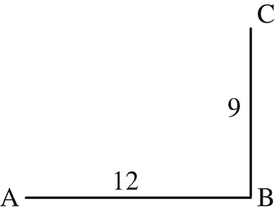
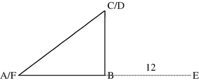
  • (b) The direct distance between cities A and C can be calculated according to Pythagoras’ theorem as $\sqrt{12^2+{9}^2}=\sqrt{144+81}=\sqrt{225}=15$. Hence, the distance matrix becomes $\left(\begin{array}{ccc}0& 12& 15\\ {}12& 0& 9\\ {}15& 9& 0\end{array}\right)$.

  • (c)

    

• 5.2. The sum and difference of the pairs of matrices are:

  • (a) $\left(\begin{array}{cc}5& 2\\ {}2& 15\end{array}\right)$ and $\left(\begin{array}{cc}1& 6\\ {}-4& 1\end{array}\right)$

  • (b) $\left(\begin{array}{ccc}7& -4& 6\\ {}-1& 4& 1\\ {}-4& 6& 2\end{array}\right)$ and $\left(\begin{array}{ccc}-1& -10& 2\\ {}-3& 8& 9\\ {}6& -10& -20\end{array}\right)$

  • (c) $\left(\begin{array}{c}2\kern1em 1.6\kern1em -1\\ {}5.1\kern0.5em 1\kern0.5em -2\end{array}\right)$ and $\left(\begin{array}{c}0.4\kern1em 4.8\kern1em -2\\ {}1.7\kern0.5em 3.6\kern0.5em -4.4\end{array}\right)$

• 5.3.

  • (a) $\left(\begin{array}{c}6\\ {}7\\ {}8\end{array}\kern1em \begin{array}{c}0\\ {}-4\\ {}10\end{array}\right)$

  • (b) $\left(\begin{array}{cc}3.5& 0\\ {}2.9& 0.7\end{array}\right)$

• 5.4. Possibilities for multiplication are AB, AC, BD, CB and DA.

• 5.5.

  • (a) 2 × 7

  • (b) 2 × 1

  • (c) × 1

• 5.6.

  • (a) AB = $\left(\begin{array}{cc}18& 22\\ {}22& 58\end{array}\right)$, BA = $\left(\begin{array}{cc}8& -8\\ {}2& 68\end{array}\right)$

  • (b) BA = $\left(\begin{array}{c}8\\ {}3\\ {}-20\end{array}\kern1em \begin{array}{c}-14\\ {}-11\\ {}61\end{array}\right)$

  • (c) no matrix product possible

• 5.7.

  • (a) $\left(\begin{array}{cc}2& 6\\ {}-4& 1\end{array}\right)$

  • (b) $\left(\begin{array}{c}2.8\kern1em -2.7\kern1em 0.5\\ {}12\kern0.5em -0.7\kern0.5em -4\end{array}\right)$

• 5.8.

  • (a) $\left(\begin{array}{cc}3& -1\\ {}-3& 1\end{array}\kern1em \begin{array}{cc}4& 6\\ {}-4& 3\end{array}\kern1em \begin{array}{cc}-2& 8\\ {}-1& 4\end{array}\right)$

  • (b) $\left(\begin{array}{ccc}0& -2& -4\\ {}-6& -8& -10\\ {}-12& -14& -16\end{array}\kern1em \begin{array}{ccc}0& -3& -6\\ {}-9& -12& -15\\ {}-18& -21& -24\end{array}\right)$

• 5.9.

  • (a) symmetric, logical

  • (b) sparse, upper-triangular

  • (c) skew-symmetric

  • (d) upper-triangular

  • (e) diagonal, sparse

  • (f) identity, diagonal, logical, sparse

• 5.10.

  • (a) $\left(\begin{array}{ccc}1& i& 5\\ {}2& 1& 4-5i\\ {}3& -3+2i& 3\end{array}\right)$

  • (b) $\left(\begin{array}{ccc}1& -1& 5\\ {}2& 1& 4\\ {}3& -3& 0\end{array}\right)$

  • (c) $\left(\begin{array}{ccc}4& 19-i& 8i\\ {}0& -3& -11+i\\ {}3+2i& -3& 17\end{array}\right)$

• 5.11. Using Cramer’s rule we find that $x=\frac{D_x}{D}=\left|\begin{array}{cc}c& b\\ {}f& e\end{array}\right|/\left|\begin{array}{cc}a& b\\ {}d& e\end{array}\right|=\frac{ce- bf}{ae- bd}$ and $y=\frac{D_y}{D}=\left|\begin{array}{cc}a& c\\ {}d& f\end{array}\right|/\left|\begin{array}{cc}a& b\\ {}d& e\end{array}\right|=\frac{af- cd}{ae- bd}$. From Sect. 5.3.1 we obtain that the inverse of the matrix $\left(\begin{array}{cc}a& b\\ {}d& e\end{array}\right)$ is equal to $\frac{1}{ae- bd}\left(\begin{array}{cc}e& -b\\ {}-d& a\end{array}\right)$ and the solution to the system of linear equations is $\frac{1}{ae- bd}\left(\begin{array}{cc}e& -b\\ {}-d& a\end{array}\right)\left(\begin{array}{c}c\\ {}f\end{array}\right)=\left(\begin{array}{c}\left( ce- bf\right)/\left( ae- bd\right)\\ {}\left( af- cd\right)/\left( ae- bd\right)\end{array}\right)$ which is the same as the solution obtained using Cramer’s rule.

• 5.12.

  • (a) x =  − 11, $y=-5\frac{3}{5}$

  • (b) $D=\left|\begin{array}{ccc}4& -2& -2\\ {}2& 8& 4\\ {}30& 12& -4\end{array}\right|=4\left(8\cdot -4-4\cdot 12\right)-\cdot -2\left(2\cdot -4-30\cdot 4\right)+\cdot -2\left(2\cdot 12-30\cdot 8\right)=-144$

$$ {D}_x=\left|\begin{array}{ccc}10& -2& -2\\ {}32& 8& 4\\ {}24& 12& -4\end{array}\right|=-1632{D}_y=\left|\begin{array}{ccc}4& 10& -2\\ {}2& 32& 4\\ {}30& 24& -4\end{array}\right|=2208 $$

$$ {D}_z=\left|\begin{array}{ccc}4& -2& 10\\ {}2& 8& 32\\ {}30& 12& 24\end{array}\right|=-4752 $$

• Thus, $x=\frac{D_x}{D}=\frac{-1632}{-144}=11\frac{1}{3}$, $y=\frac{D_y}{D}=\frac{2208}{-144}=-15\frac{1}{3}$ and $z=\frac{D_z}{D}=\frac{-4752}{-144}=33$

• 5.13.

  • (a) x = 4, y = 0

  • (b) x = 2, y = − 1, z = 1

• 5.14. This shearing matrix shears along the x-axis and leaves y-coordinates unchanged (see Sect. 5.2.2). Hence, all vectors along the x-axis remain unchanged due to this transformation. The eigenvector is thus $\left(\begin{array}{c}1\\ {}0\end{array}\right)$ with eigenvalue 1 (since the length of the eigenvector is unchanged due to the transformation).

• 5.15.

  • (a) λ₁ = 7 with eigenvector $\left(\begin{array}{c}1\\ {}0\\ {}0\end{array}\right)$ (x = x, y = 0, z = 0), λ₂ =  − 19 with eigenvector $\left(\begin{array}{c}0\\ {}1\\ {}0\end{array}\right)$ (x = 0, y = y, z = 0) and λ₃ = 2 with eigenvector $\left(\begin{array}{c}0\\ {}0\\ {}1\end{array}\right)$ (x = 0, y = 0, z = z).

  • (b) λ = 3 (double) with eigenvector $\left(\begin{array}{c}1\\ {}1\end{array}\right)$ (y = x).

  • (c) λ₁ = 1 with eigenvector $\left(\begin{array}{c}-1\\ {}1\\ {}1\end{array}\right)$ (x = −z, y = z), λ₂ =  − 1 with eigenvector $\left(\begin{array}{c}1\\ {}1\\ {}5\end{array}\right)$ (5x = z, 5y = z) and λ₃ = 3 with eigenvector $\left(\begin{array}{c}1\\ {}1\\ {}1\end{array}\right)$ (x = y = z).

  • (d) λ₁ = 3 with eigenvector $\left(\begin{array}{c}1\\ {}-2\end{array}\right)$ (y = −2x) and λ₂ = 7 with eigenvector $\left(\begin{array}{c}1\\ {}2\end{array}\right)$ (y = 2x).

• 5.16.

  • (a) To determine the SVD, we first determine the eigenvalues and eigenvectors of M^TM to get the singular values and right-singular vectors of M. Thus, we determine its characteristic equation as the determinant

    $$ {\displaystyle \begin{array}{l}\left|\left(\begin{array}{cc}2& 1\\ {}1& 2\end{array}\right)\left(\begin{array}{cc}2& 1\\ {}1& 2\end{array}\right)-\lambda \left(\begin{array}{cc}1& 0\\ {}0& 1\end{array}\right)\right|=\left|\left(\begin{array}{cc}5& 4\\ {}4& 5\end{array}\right)-\lambda \left(\begin{array}{cc}1& 0\\ {}0& 1\end{array}\right)\right|=\\ {}\left|\left(\begin{array}{cc}5-\lambda & 4\\ {}4& 5-\lambda \end{array}\right)\right|={\left(5-\lambda \right)}^2-16={\lambda}^2-10\lambda +9=\left(\lambda -1\right)\left(\lambda -9\right)\end{array}} $$

• Thus, the singular values are ${\sigma}_1=\sqrt{9}=3$ and ${\sigma}_1=\sqrt{1}=1$ and $\Sigma =\left(\begin{array}{cc}3& 0\\ {}0& 1\end{array}\right)$.

• The eigenvector belonging to the first eigenvalue of M^TM follows from:

$$ {\displaystyle \begin{array}{l}\left(\begin{array}{cc}5& 4\\ {}4& 5\end{array}\right)\left(\begin{array}{c}x\\ {}y\end{array}\right)=9\left(\begin{array}{c}x\\ {}y\end{array}\right)\Rightarrow \left(\begin{array}{c}5x+4y\\ {}4x+5y\end{array}\right)=\left(\begin{array}{c}9x\\ {}9y\end{array}\right)\\ {}\Rightarrow 5x+4y=9x\wedge 4x+5y=9y\\ {}\Rightarrow -4x+4y=0\wedge 4x-4y=0\\ {}\Rightarrow x=y\\ {}\Rightarrow \left(\begin{array}{c}x\\ {}y\end{array}\right)=\left(\begin{array}{c}1\\ {}1\end{array}\right)\end{array}} $$

• To determine the first column of V, this eigenvector must be normalized (divided by its length; see Sect. 4.2.2.1) and thus ${\overrightarrow{v}}_1=\frac{1}{\sqrt{2}}\left(\begin{array}{c}1\\ {}1\end{array}\right)$.

• Similarly, the eigenvector belonging to the second eigenvalue of M^TM can be derived to be ${\overrightarrow{v}}_2=\frac{1}{\sqrt{2}}\left(\begin{array}{c}1\\ {}-1\end{array}\right)$, making $V=\frac{1}{\sqrt{2}}\left(\begin{array}{cc}1& 1\\ {}1& -1\end{array}\right)$. In this case, ${\overrightarrow{v}}_1$ and ${\overrightarrow{v}}_2$ are already orthogonal (see Sect. 4.2.2.1), making further adaptations to arrive at an orthonormal set of eigenvectors unnecessary.

• To determine U we use that ${\overrightarrow{u}}_1=\frac{1}{\sigma_1}M{\overrightarrow{v}}_1=\frac{1}{3}\left(\begin{array}{cc}2& 1\\ {}1& 2\end{array}\right)\frac{1}{\sqrt{2}}\left(\begin{array}{c}1\\ {}1\end{array}\right)=\frac{1}{\sqrt{2}}\left(\begin{array}{c}1\\ {}1\end{array}\right)$ and ${\overrightarrow{u}}_2=\frac{1}{\sigma_2}M{\overrightarrow{v}}_2=\frac{1}{1}\left(\begin{array}{cc}2& 1\\ {}1& 2\end{array}\right)\frac{1}{\sqrt{2}}\left(\begin{array}{c}1\\ {}-1\end{array}\right)=\frac{1}{\sqrt{2}}\left(\begin{array}{c}1\\ {}-1\end{array}\right)$, making $U=\frac{1}{\sqrt{2}}\left(\begin{array}{cc}1& 1\\ {}1& -1\end{array}\right)$. You can now verify yourself that indeed M = UΣV∗.

  • (b) Taking a similar approach, we find that

    $$ U=\left(\begin{array}{cc}1& 0\\ {}0& 1\end{array}\right),\Sigma =\left(\begin{array}{cc}2& 0\\ {}0& 1\end{array}\right)\ \mathrm{and}\ V=\left(\begin{array}{cc}1& 0\\ {}0& 1\end{array}\right). $$

• 5.17. If M = UΣV∗ and using that both U and V are unitary (see Table 5.1), then MM∗ = UΣV∗(UΣV∗)∗ = UΣV∗VΣU∗ = UΣ²U∗. Right-multiplying both sides of this equation with U and then using that Σ² is diagonal, yields MM∗U = UΣ² = Σ²U. Hence, the columns of U are eigenvectors of MM^* (with eigenvalues equal to the diagonal elements of Σ²).

Glossary

Adjacency matrix

Matrix with binary entries (i,j) describing the presence (1) or absence (0) of a path between nodes i and j.

Adjoint

Transpose of the cofactor matrix.

Airfoil

Shape of an airplane wing, propeller blade or sail.

Ataxia

A movement disorder or symptom involving loss of coordination.

Basis vector

A set of (N-dimensional) basis vectors is linearly independent and any vector in N-dimensional space can be built as a linear combination of these basis vectors.

Boundary conditions

Constraints for a solution to an equation on the boundary of its domain.

Cofactor matrix

The (i,j)-element of this matrix is given by the determinant of the matrix that remains when the i-th row and j-th column are removed from the original matrix, multiplied by −1 if i + j is odd.

Conjugate transpose

Generalization of transpose; a transformation of a matrixAindicated byA^*with elements defined by ${\left({A}^{\ast}\right)}_{ij}={\overline{a}}_{ji}$_.

Dense matrix

A matrix whose elements are almost all non-zero.

Determinant

Can be seen as a scaling factor when calculating the inverse of a matrix.

Diagonalization

Decomposition of a matrix M such that it can be written as M = VDV − ¹ where V is an invertible matrix and D is a diagonal matrix.

Diagonal matrix

A matrix with only non-zero elements on the diagonal and zeroes elsewhere.

Discretize

To represent an equation on a grid.

EEG

Electroencephalography; a measurement of electrical brain activity.

Eigendecomposition

To determine the eigenvalues and eigenvectors of a matrix.

Element

As in ‘matrix element’: one of the entries in a matrix.

Gaussian

Normally distributed.

Graph

A collection of nodes or vertices with paths or edges between them whenever the nodes are related in some way.

Hadamard product

Element-wise matrix product.

Identity matrix

A squarematrix with ones on the diagonal and zeroes elsewhere, often referred to asI. The identity matrix is a special diagonal matrix.

Independent component analysis

A method to determine independent components of non-Gaussian signals by minimizing higher order moments of the data.

Inverse

The matrix A⁻¹ such that AA⁻¹ = A⁻¹A = I.

Invertable

A matrix that has an inverse.

Kronecker product

Generalization of the outer product (or tensor product or dyadic product) for vectors to matrices.

Kurtosis

Fourth-order moment of data, describing how much of the data variance is in the tail of its distribution.

Laplace equation

Partial differential equation describing the behavior of potential fields.

Left-singular vector

Columns of U in the SVD of M: M = UΣV^∗_.

Leslie matrix

Matrix with probabilities to transfer from one age class to the next in a population ecological model of population growth.

Logical matrix

A matrix that only contains zeroes and ones (also: binary or Boolean matrix).

Matrix

A rectangular array of (usually) numbers.

Network theory

The study of graphs as representing relations between different entities, such as in a social network, brain network, gene network etcetera.

Order

Size of a matrix.

Orthonormal

Orthogonal vectors of length 1.

Partial differential equation

An equation that contains functions of multiple variables and their partial derivatives (see also Chap. 6).

Principal component analysis

Method that transforms data to a new coordinate system such that the largest variance is found along the first new coordinate (first PC), the then largest variance is found along the second new coordinate (second PC) etcetera.

Right-singular vector

Columns of V in the SVD of M: M = UΣV∗

Root

Here: a value of λ that makes the characteristic polynomial |M − λI| of the matrix M equal to zero.

Scalar function

Function with scalar values.

Shearing

To shift along one axis.

Singular value

Diagonal elements of Σ in the SVD of M: M = UΣV∗_.

Singular value decomposition

The decomposition of an m × n rectangular matrix M into a product of three matrices such that M = UΣV∗ where U is a unitary m × m matrix, Σ an m × n diagonal matrix with non-negative real entries and V another unitary n × n matrix.

Skewness

Third-order moment of data, describing asymmetry of its distribution.

Skew-symmetric matrix

A matrix A for which a_ij =  − a_ji.

Sparse matrix

A matrix with most of its elements equal to zero.

Stationary

Time-dependent data for which the most important statistical properties (such as mean and variance) do not change over time.

Symmetric matrix

A matrix A that is symmetric around the diagonal, i.e. for which a_ij = a_ji.

Transformation

Here: linear transformation as represented by matrices. A function mapping a set onto itself (e.g. 2D space onto 2D space).

Transpose

A transformation of a matrix A indicated by A^T with elements defined by (A^T)_ij = a_ji.

Triangular matrix

A diagonal matrixextended with non-zero elements only above or only below the diagonal.

Unit matrix

Identity matrix.