Proving Non-Termination and Lower Runtime Bounds with LoAT (System Description)

Abstract

We present the Loop Acceleration Tool (LoAT), a powerful tool for proving non-termination and worst-case lower bounds for programs operating on integers. It is based on the novel calculus from [10, 11] for loop acceleration, i.e., transforming loops into non-deterministic straight-line code, and for finding non-terminating configurations. To implement it efficiently, LoAT uses a new approach based on unsat cores. We evaluate LoAT’s power and performance by extensive experiments.

Funded by the Deutsche Forschungsgemeinschaft (DFG, German Research Foundation) - 235950644 (Project GI 274/6-2).

1 Introduction

Efficiency is one of the most important properties of software. Consequently, automated complexity analysis is of high interest to the software verification community. Most research in this area has focused on deducing upper bounds on the worst-case complexity of programs. In contrast, the Loop Acceleration Tool LoAT aims to find performance bugs by deducing lower bounds on the worst-case complexity of programs operating on integers. Since non-termination implies the lower bound $\infty$, LoAT is also equipped with non-termination techniques.

LoAT is based on loop acceleration [4, 5, 9,10,11, 15], which replaces loops by non-deterministic code: The resulting program chooses a value n, representing the number of loop iterations in the original program. To be sound, suitable constraints on n are synthesized to ensure that the original loop allows for at least n iterations. Moreover, the transformed program updates the program variables to the same values as n iterations of the original loop, but it does so in a single step. To achieve that, the loop body is transformed into a closed form, which is parameterized in n. In this way, LoAT is able to compute symbolic under-approximations of programs, i.e., every execution path in the resulting transformed program corresponds to a path in the original program, but not necessarily vice versa. In contrast to many other techniques for computing under-approximations, the symbolic approximations of LoAT cover infinitely many runs of arbitrary length.

Contributions: The main new feature of the novel version of LoAT presented in this paper is the integration of the loop acceleration calculus from [10, 11], which combines different loop acceleration techniques in a modular way, into LoAT’s framework. This enables LoAT to use the loop acceleration calculus for the analysis of full integer programs, whereas the standalone implementation of the calculus from [10, 11] was only applicable to single loops without branching in the body. To control the application of the calculus, we use a new technique based on unsat cores (see Sect. 5). The new version of LoAT is evaluated in extensive experiments. See [14] for all proofs.

2 Preliminaries

Let $\mathcal {L}\supseteq \{ main \}$ be a finite set of locations, where $main$ is the canonical start location (i.e., the entry point of the program), and let $\vec {x} \mathrel {\mathop :}=[x_1,\ldots ,x_d]$ be the vector of program variables. Furthermore, let $\mathcal{TV}\mathcal{}$ be a countably infinite set of temporary variables, which are used to model non-determinism, and let $\sup \mathbb {Z}\mathrel {\mathop :}=\infty$. We call an arithmetic expression e an integer expression if it evaluates to an integer when all variables in e are instantiated by integers. LoAT analyzes tail-recursive programs operating on integers, represented as integer transition systems (ITSs), i.e., sets of transitions $f(\vec {x}) \mathop {\rightarrow }\nolimits ^{p} g(\vec {a}) \left[ \varphi \right]$ where $f,g \in \mathcal {L}$, the update $\vec {a}$ is a vector of d integer expressions over $\mathcal{TV}\mathcal{}\cup \vec {x}$, the cost p is either an arithmetic expression over $\mathcal{TV}\mathcal{}\cup \vec {x}$ or $\infty$, and the guard $\varphi$ is a conjunction of inequations over integer expressions with variables from $\mathcal{TV}\mathcal{}\cup \vec {x}$.¹ For example, consider the loop on the left and the corresponding transition $t_{ loop }$ on the right.

Here, the cost 1 instructs LoAT to use the number of loop iterations as cost measure. LoAT allows for arbitrary user defined cost measures, since the user can choose any polynomials over the program variables as costs. LoAT synthesizes transitions with cost $\infty$ to represent non-terminating runs, i.e., such transitions are not allowed in the input.

A configuration is of the form $f(\vec {c})$ with $f \in \mathcal {L}$ and $\vec {c} \in \mathbb {Z}^d$. For any entity $s \notin \mathcal {L}$ and any arithmetic expressions $\vec {b} = [b_1,\ldots ,b_d]$, let $s(\vec {b})$ denote the result of replacing each variable $x_i$ in s by $b_i$, for all $1 \le i \le d$. Moreover, $\mathcal {V}\! ars (s)$ denotes the program variables and $\mathcal{TV}\mathcal{}(s)$ denotes the temporary variables occurring in s. For an integer transition system $\mathcal {T}$, a configuration $f(\vec {c})$ evaluates to $g(\vec {c}\,')$ with cost $k \in \mathbb {Z}\cup \{\infty \}$, written $f(\vec {c}) \mathop {\rightarrow }\nolimits ^{k}_\mathcal {T}g(\vec {c}\,')$, if there exist a transition $f(\vec {x}) \mathop {\rightarrow }\nolimits ^{p} g(\vec {a}) \left[ \varphi \right] \in \mathcal {T}$ and an instantiation of its temporary variables with integers such that the following holds:

$$ \varphi (\vec {c}) \wedge \vec {c}\,' = \vec {a}(\vec {c}) \wedge k = p(\vec {c}). $$

As usual, we write if $f(\vec {c})$ evaluates to $g(\vec {c}\,')$ in arbitrarily many steps, and the sum of the costs of all steps is k. We omit the costs if they are irrelevant. The derivation height of $f(\vec {c})$ is

and the runtime complexity of $\mathcal {T}$ is

$$ rc _\mathcal {T}(n) \mathrel {\mathop :}=\sup \{ dh _\mathcal {T}( main (c_1,\ldots ,c_d)) \mid |c_1| + \ldots + |c_d| \le n\}. $$

$\mathcal {T}$ terminates if no configuration $main (\vec {c})$ admits an infinite ${\mathop {\rightarrow }\nolimits ^{}_\mathcal {T}}$-sequence and $\mathcal {T}$ is finitary if no configuration $main (\vec {c})$ admits a ${\mathop {\rightarrow }\nolimits ^{}_\mathcal {T}}$-sequence with cost $\infty$. Otherwise, $\vec {c}$ is a witness of non-termination or a witness of infinitism, respectively. Note that termination implies finitism for ITSs where no transition has cost $\infty$. However, our approach may transform non-terminating ITSs into terminating, infinitary ITSs, as it replaces non-terminating loops by transitions with cost $\infty$.

3 Overview of LoAT

The goal of LoAT is to compute a lower bound on $rc _\mathcal {T}$ or even prove non-termination of $\mathcal {T}$. To this end, it repeatedly applies program simplifications, so-called processors. When applying them with a suitable strategy (see [8, 9]), one eventually obtains simplified transitions of the form $main (\vec {x}) \mathop {\rightarrow }\nolimits ^{p} f(\vec {a}) \left[ \varphi \right]$ where $f \ne main$. As LoAT’s processors are sound for lower bounds (i.e., if they transform $\mathcal {T}$ to $\mathcal {T}'$, then $dh _\mathcal {T}\ge dh _{\mathcal {T}'}$), such a simplified transition gives rise to the lower bound $I_{\varphi } \cdot p$ on $dh _\mathcal {T}( main (\vec {x}))$ (where $I_{\varphi }$ denotes the indicator function of $\varphi$, which is 1 for values where $\varphi$ holds and 0 otherwise). This bound can be lifted to $rc _\mathcal {T}$ by solving a so-called limit problem, see [9].

LoAT’s processors are also sound for non-termination, as they preserve finitism. So if $p = \infty$, then it suffices to prove satisfiability of $\varphi$ to prove infinitism, which implies non-termination of the original ITS, where transitions with cost $\infty$ are forbidden (see Sect. 2). LoAT’s most important processors are:

• Loop Acceleration (Sect. 4) transforms a simple loop, i.e., a single transition $f(\vec {x}) \mathop {\rightarrow }\nolimits ^{p} f(\vec {a}) \left[ \varphi \right]$, into a non-deterministic transition that can simulate several loop iterations in one step. For example, loop acceleration transforms $t_{ loop }$ to

  

  where $n \in \mathcal{TV}\mathcal{}$, i.e., the value of n can be chosen non-deterministically.

• Instantiation [9, Theorem 3.12] replaces temporary variables by integer expressions. For example, it could instantiate n with x in $t_{ loop ^n}$, resulting in

  

• Chaining [9, Theorem 3.18] combines two subsequent transitions into one transition. For example, chaining combines the transitions

  $$\begin{aligned} main (x)&\mathop {\rightarrow }\nolimits ^{1} f(x)\\ \text {and} t_{ loop ^x} \text {to} \quad main (x)&\mathop {\rightarrow }\nolimits ^{x+1} f(0) \left[ x > 0\right] . \end{aligned}$$

• Nonterm (Sect. 6) searches for witnesses of non-termination, characterized by a formula $\psi$. So it turns, e.g.,

  

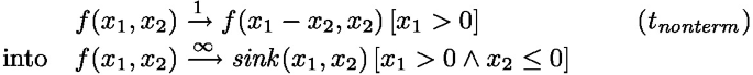
  (where $sink \in \mathcal {L}$ is fresh), as each $\vec {c} \in \mathbb {Z}^2$ with $c_1 > 0 \wedge c_2 \le 0$ witnesses non-termination of $t_{ nonterm }$, i.e., here $\psi$ is $x_1 > 0 \wedge x_2 \le 0$.

Intuitively, LoAT uses Chaining to transform non-simple loops into simple loops. Instantiation resolves non-determinism heuristically and thus reduces the number of temporary variables, which is crucial for scalability. In addition to these processors, LoAT removes transitions after processing them, as explained in [9]. See [8, 9] for heuristics and a suitable strategy to apply LoAT’s processors.

4 Modular Loop Acceleration

For Loop Acceleration, LoAT uses conditional acceleration techniques [10]. Given two formulas $\xi$ and , and a loop with update $\vec {a}$, a conditional acceleration technique yields a formula which implies that $\xi$ holds throughout n loop iterations (i.e., $\xi$ is an n-invariant), provided that is an n-invariant, too. In the following, let $\vec {a}^0(\vec {x}) \mathrel {\mathop :}=\vec {x}$ and $\vec {a}^{m+1}(\vec {x}) \mathrel {\mathop :}=\vec {a}(\vec {a}^m(\vec {x})) = \vec {a}[\vec {x}/\vec {a}^m(\vec {x})]$.

Definition 1

(Conditional Acceleration Technique). A function $accel$ is a conditional acceleration technique if the following implication holds for all formulas $\xi$ and with variables from $\mathcal{TV}\mathcal{}\cup \vec {x}$, all updates $\vec {a}$, all $n>0$, and all instantiations of the variables with integers:

The prerequisite is ensured by previous acceleration steps, i.e., is initially $\top$ (true), and it is refined by conjoining a part $\xi$ of the loop guard in each acceleration step. When formalizing acceleration techniques, we only specify the result of $accel$ for certain arguments $\xi$, , and $\vec {a}$, and assume (false) otherwise.

Definition 2

(LoAT’s Conditional Acceleration Techniques [10, 11]).

The above five techniques are taken from [10, 11], where only deterministic loops are considered (i.e., there are no temporary variables). Lifting them to non-deterministic loops in a way that allows for exact conditional acceleration techniques (which capture all possible program runs) is non-trivial and beyond the scope of this paper. Thus, we sacrifice exactness and treat temporary variables like additional constant program variables whose update is the identity, resulting in a sound under-approximation (that captures a subset of all possible runs).

So essentially, Increase and Decrease handle inequations $t > 0$ in the loop guard where t increases or decreases (weakly) monotonically when applying the loop’s update. The canonical examples where Increase or Decrease applies are

$$ f(x,\ldots ) \rightarrow f(x+1,\ldots ) \left[ x>0 \wedge \ldots \right] \quad \text {or} \quad f(x,\ldots ) \rightarrow f(x-1,\ldots ) \left[ x>0 \wedge \ldots \right] , $$

respectively. Eventual Decrease applies if t never increases again once it starts to decrease. The canonical example is $f(x,y,\ldots ) \rightarrow f(x+y,y-1,\ldots ) \left[ x>0 \wedge \ldots \right]$. Similarly, Eventual Increase applies if t never decreases again once it starts to increase. Fixpoint can be used for inequations $t > 0$ that do not behave (eventually) monotonically. It should only be used if is satisfiable.

LoAT uses the acceleration calculus of [10]. It operates on acceleration problems , where $\psi$ (which is initially $\top$) is repeatedly refined. When it stops, $\psi$ is used as the guard of the resulting accelerated transition. The formulas and $\widehat{\varphi }$ are the parts of the loop guard that have already or have not yet been handled, respectively. So is initially $\top$, and $\widehat{\varphi }$ and $\vec {a}$ are initialized with the guard $\varphi$ and the update of the loop $f(\vec {x}) \mathop {\rightarrow }\nolimits ^{p} f(\vec {a}) \left[ \varphi \right]$ under consideration, i.e., the initial acceleration problem is $\llbracket \top \, |\, \top \,|\, \varphi \rrbracket _{\vec {a}}$. Once $\widehat{\varphi }$ is $\top$, the loop is accelerated to $f(\vec {x}) \mathop {\rightarrow }\nolimits ^{q} f(\vec {a}^n(\vec {x})) \left[ \psi \wedge n > 0\right]$, where the cost q and a closed form for $\vec {a}^n(\vec {x})$ are computed by the recurrence solver PURRS [2].

Definition 3

(Acceleration Calculus for Conjunctive Loops). The relation ${\leadsto }$ on acceleration problems is defined as

So to accelerate a loop, one picks a not yet handled part $\xi$ of the guard in each step. When accelerating $f(\vec {x}) \mathop {\rightarrow }\nolimits ^{} f(\vec {a}) \left[ \xi \right]$ using a conditional acceleration technique $accel$, one may assume . The result of $accel$ is conjoined to the result $\psi _1$ computed so far, and $\xi$ is moved from the third to the second component of the problem, i.e., to the already handled part of the guard.

Example 4

(Acceleration Calculus). We show how to accelerate the loop

The closed form $\vec {a}^n(x) = (x - n \cdot y, y)$ can be computed via recurrence solving. Similarly, the cost $(x + \frac{y}{2}) \cdot n - \frac{y}{2} \cdot n^2$ of n loop iterations is obtained by solving the following recurrence relation (where $c^{(n)}$ and $x^{(n)}$ denote the cost and the value of x after n applications of the transition, respectively).

$$ c^{(n)} = c^{(n-1)} + x^{(n-1)} = c^{(n-1)} + x - (n-1) \cdot y \qquad \text {and} \qquad c^{(1)} = x. $$

The guard is computed as follows:

$$\begin{aligned} \llbracket \top \, |\, \top \,|\, x> 0 \wedge y \ge 0 \rrbracket _{\vec {a}}&\leadsto \llbracket y \ge 0\, |\, y \ge 0 \,|\, x> 0 \rrbracket _{\vec {a}} \\&\leadsto \llbracket y \ge 0 \wedge x - (n - 1) \cdot y> 0\, |\, y \ge 0 \wedge x > 0 \,|\, \top \rrbracket _{\vec {a}}. \end{aligned}$$

In the $1^{st}$ step, we have $\xi = (y \ge 0)$ and $accel _ inc (y \ge 0, \top , \vec {a}) = (y \ge 0)$. In the $2^{nd}$ step, we have $\xi = (x > 0)$ and $accel _ dec (x>0,y \ge 0,\vec {a}) = (x-(n-1) \cdot y > 0)$. So the inequation $x - (n - 1) \cdot y > 0$ ensures n-invariance of $x>0$.

5 Efficient Loop Acceleration Using Unsat Cores

Each attempt to apply a conditional acceleration technique other than Fixpoint requires proving an implication, which is implemented via SMT solving by proving unsatisfiability of its negation. For Fixpoint, satisfiability of is checked via SMT. So even though LoAT restricts $\xi$ to atoms, up to $\varTheta (m^2)$ attempts to apply a conditional acceleration technique are required to accelerate a loop whose guard contains m inequations using a naive strategy ($5 \cdot m$ attempts for the $1^{st}$ ${\leadsto }$-step, $5 \cdot (m-1)$ attempts for the $2^{nd}$ step, ...).

To improve efficiency, LoAT uses a novel encoding that requires just $5 \cdot m$ attempts. For any $\alpha \in AT_ imp = \{ inc , dec , { ev \text {-} dec }, { ev \text {-} inc }\}$, let be the implication that has to be valid in order to apply $accel _\alpha$, whose premise is of the form . Instead of repeatedly refining , LoAT tries to prove validity² of $encode _{\alpha ,\xi } \mathrel {\mathop :}= encode _\alpha ( \xi , \varphi \setminus \{\xi \}, \vec {a})$ for each $\alpha \in AT_ imp$ and each $\xi \in \varphi$, where $\varphi$ is the (conjunctive) guard of the transition that should be accelerated. Again, proving validity of an implication is equivalent to proving unsatisfiability of its negation. So if validity of $encode _{\alpha ,\xi }$ can be shown, then SMT solvers can also provide an unsat core for $\lnot encode _{\alpha ,\xi }$.

Definition 5

(Unsat Core). Given a conjunction $\psi$, we call each unsatisfiable subset of $\psi$ an unsat core of $\psi$.

Theorem 6 shows that when handling an inequation $\xi$, one only has to require n-invariance for the elements of $\varphi \setminus \{\xi \}$ that occur in an unsat core of $\lnot encode _{\alpha ,\xi }$. Thus, an unsat core of $\lnot encode _{\alpha ,\xi }$ can be used to determine which prerequisites are needed for the inequation $\xi$. This information can then be used to find a suitable order for handling the inequations of the guard. Thus, in this way one only has to check (un)satisfiability of the $4 \cdot m$ formulas $\lnot encode _{\alpha ,\xi }$. If no such order is found, then LoAT either fails to accelerate the loop under consideration, or it resorts to using Fixpoint, as discussed below.

Theorem 6

(Unsat Core Induces ${\leadsto }$-Step). Let $deps _{\alpha ,\xi }$ be the intersection of $\varphi \setminus \{\xi \}$ and an unsat core of $\lnot encode _{\alpha ,\xi }$. If implies $deps _{\alpha ,\xi }$, then .

Example 7

(Controlling Acceleration Steps via Unsat Cores). Reconsider Example 4. Here, LoAT would try to prove, among others, the following implications:

$$\begin{aligned} encode _{ dec ,x>0}&\quad = \quad (x-y>0 \wedge y> 0) \implies x > 0 \end{aligned}$$

(1)

$$\begin{aligned} encode _{ inc ,y>0}&\quad = \quad (y>0 \wedge x> 0) \implies y > 0 \end{aligned}$$

(2)

To do so, it would try to prove unsatisfiability of $\lnot encode _{\alpha ,\xi }$ via SMT. For (1), we get $\lnot encode _{ dec ,x>0} = (x-y> 0 \wedge y > 0 \wedge x \le 0)$, whose only unsat core is $\lnot encode _{ dec ,x>0}$, and its intersection with $\varphi \setminus \{x> 0\} = \{y > 0\}$ is $\{y > 0\}$.

For (2), we get $\lnot encode _{ inc ,y>0} = (y> 0 \wedge x > 0 \wedge y \le 0)$, whose minimal unsat core is $y > 0 \wedge y \le 0$, and its intersection with $\varphi \setminus \{y> 0\} = \{x > 0\}$ is empty. So by Theorem 6, we have $accel _ inc (y>0, \top , \vec {a}) = accel _ inc (y>0, x>0, \vec {a})$.

In this way, validity of $encode _{\alpha _1,x>0}$ and $encode _{\alpha _2,y>0}$ is proven for all $\alpha _1 \in AT_ imp \setminus \{ inc \}$ and all $\alpha _2 \in AT_ imp$. However, the premise $x \le x-y \wedge y > 0$ of $encode _{{ ev \text {-} inc },x>0}$ is unsatisfiable and thus a corresponding acceleration step would yield a transition with unsatisfiable guard. To prevent that, LoAT only uses a technique $\alpha \in AT_ imp$ for $\xi$ if the premise of $encode _{\alpha ,\xi }$ is satisfiable.

So for each inequation $\xi$ from $\varphi$, LoAT synthesizes up to 4 potential ${\leadsto }$-steps corresponding to $accel _\alpha (\xi , deps _{\alpha ,\xi }, \vec {a})$, where $\alpha \in AT_ imp$. If validity of $encode _{\alpha ,\xi }$ cannot be shown for any $\alpha \in AT_ imp$, then LoAT tries to prove satisfiability of $accel _ fp (\xi , \top , \vec {a})$ to see if Fixpoint should be applied. Note that the $2^{nd}$ argument of $accel _ fp$ is irrelevant, i.e., Fixpoint does not benefit from previous acceleration steps and thus ${\leadsto }$-steps that use it do not have any dependencies.

It remains to find a suitably ordered subset S of m ${\leadsto }$-steps that constitutes a successful ${\leadsto }$-sequence. In the following, we define $AT\mathrel {\mathop :}=AT_ imp \cup \{ fp \}$ and we extend the definition of $deps _{\alpha ,\xi }$ to the case $\alpha = fp$ by defining $deps _{ fp ,\xi } \mathrel {\mathop :}=\varnothing$.

Lemma 8

Let $C \subseteq AT\times \varphi$ be the smallest set such that $(\alpha ,\xi ) \in C$ implies

• (a) if $\alpha \in AT_ imp$, then $encode _{\alpha ,\xi }$ is valid and its premise is satisfiable,

• (b) if $\alpha = fp$, then $accel _ fp (\xi , \top , \vec {a})$ is satisfiable, and

• (c) $deps _{\alpha ,\xi } \subseteq \{\xi ' \mid (\alpha ',\xi ') \in C \text { for some } \alpha ' \in AT\}$.

Let $S \mathrel {\mathop :}=\{(\alpha ,\xi ) \in C \mid \alpha \ge _{AT} \alpha ' \text { for all } (\alpha ',\xi ) \in C\}$ where ${>_{AT}}$ is the total order $inc>_{AT} dec>_{AT} { ev \text {-} dec }>_{AT} { ev \text {-} inc }>_{AT} fp$. We define $(\alpha ',\xi ') \prec (\alpha ,\xi )$ if $\xi ' \in deps _{\alpha ,\xi }$. Then ${\prec }$ is a strict (and hence, well-founded) order on S.

The order ${>_{AT}}$ in Lemma 8 corresponds to the order proposed in [10]. Note that the set C can be computed without further (potentially expensive) SMT queries by a straightforward fixpoint iteration, and well-foundedness of ${\prec }$ follows from minimality of C. For Example 7, we get

$$\begin{aligned} C = {}&\{( dec , x>0), ({ ev \text {-} dec }, x>0)\} \cup \{(\alpha , y>0) \mid \alpha \in AT\}&\text {and} \\ S = {}&\{( dec , x>0), ( inc , y>0)\} \text { with } ( inc , y>0) \; {\prec } \; ( dec , x>0). \end{aligned}$$

Finally, we can construct a valid ${\leadsto }$-sequence via the following theorem.

Theorem 9

(Finding ${\leadsto }$-Sequences). Let S be defined as in Lemma 8 and assume that for each $\xi \in \varphi$, there is an $\alpha \in AT$ such that $(\alpha , \xi ) \in S$. W.l.o.g., let $\varphi = \bigwedge _{i=1}^m \xi _i$ where $(\alpha _1, \xi _1) \prec ' \ldots \prec ' (\alpha _m, \xi _{m})$ for some strict total order ${\prec '}$ containing ${\prec }$, and let . Then for all $j \in [0,m)$, we have:

In our example, we have ${\prec '} = {\prec }$ as ${\prec }$ is total. Thus, we obtain a ${\leadsto }$-sequence by first processing $y>0$ with Increase and then processing $x>0$ with Decrease.

6 Proving Non-Termination of Simple Loops

To prove non-termination, LoAT uses a variation of the calculus from Sect. 4, see [11]. To adapt it for proving non-termination, further restrictions have to be imposed on the conditional acceleration techniques, resulting in the notion of conditional non-termination techniques, see [11, Def. 10]. We denote a ${\leadsto }$-step that uses a conditional non-termination technique with ${\leadsto _ nt }$.

Theorem 10

(Proving Non-Termination via ${\leadsto _ nt }$). Let $f(\vec {x}) \mathop {\rightarrow }\nolimits ^{} f(\vec {a}) \left[ \varphi \right] \in \mathcal {T}$. If $\llbracket \top \, |\, \top \,|\, \varphi \rrbracket _{\vec {a}} \leadsto _ nt ^* \llbracket \psi \, |\, \varphi \,|\, \top \rrbracket _{\vec {a}}$, then for every $\vec {c} \in \mathbb {Z}^d$ where $\psi (\vec {c})$ is satisfiable, the configuration $f(\vec {c})$ admits an infinite $\mathop {\rightarrow }\nolimits ^{}_{\mathcal {T}}$-sequence.

The conditional non-termination techniques used by LoAT are Increase, Eventual Increase, and Fixpoint. So non-termination proofs can be synthesized while trying to accelerate a loop with very little overhead. After successfully accelerating a loop as explained in Sect. 5, LoAT tries to find a second suitably ordered ${\leadsto }$-sequence, where it only considers the conditional non-termination techniques mentioned above. If LoAT succeeds, then it has found a ${\leadsto _ nt }$-sequence which gives rise to a proof of non-termination via Theorem 10.

7 Implementation, Experiments, and Conclusion

Our implementation in LoAT can parse three widely used formats for ITSs (see [13]), and it is configurable via a minimalistic set of command-line options:

• –timeout to set a timeout in seconds

• –proof-level to set the verbosity of the proof output

• –plain to switch from colored to monochrome proof-output

• –limit-strategy to choose a strategy for solving limit problems, see [9]

• –mode to choose an analysis mode for LoAT (complexity or non_termination)

We evaluate three versions of LoAT: LoAT ’19 uses templates to find invariants that facilitate loop acceleration for proving non-termination [8]; LoAT ’20 deduces worst-case lower bounds based on loop acceleration via metering functions [9]; and LoAT ’22 applies the calculus from [10, 11] as described in Sect. 5 and 6. We also include three other state-of-the-art termination tools in our evaluation: T2 [6], VeryMax [16], and iRankFinder [3, 7]. Regarding complexity, the only other tool for worst-case lower bounds of ITSs is LOBER [1]. However, we do not compare with LOBER, as it only analyses (multi-path) loops instead of full ITSs.

We use the examples from the categories Termination (1222 examples) and Complexity of ITSs (781 examples), respectively, of the Termination Problems Data Base [19]. All benchmarks have been performed on StarExec [18] (Intel Xeon E5-2609, 2.40GHz, 264GB RAM [17]) with a wall clock timeout of 300 s.

By the table on the left, LoAT ’22 is the most powerful tool for non-termination. The improvement over LoAT ’19 demonstrates that the calculus from [10, 11] is more powerful and efficient than the approach from [8]. The last three columns show the average, the median, and the standard deviation of the wall clock runtime, including examples where the timeout was reached.

The table on the right shows the results for complexity. The diagonal corresponds to examples where LoAT ’20 and LoAT ’22 yield the same result. The entries above or below the diagonal correspond to examples where LoAT ’22 or LoAT ’20 is better, respectively. There are 8 regressions and 79 improvements, so the calculus from [10, 11] used by LoAT ’22 is also beneficial for lower bounds.

LoAT is open source and its source code is available on GitHub [12]. See [13, 14] for details on our evaluation, related work, all proofs, and a pre-compiled binary.

References

Albert, E., Genaim, S., Martin-Martin, E., Merayo, A., Rubio, A.: Lower-bound synthesis using loop specialization and Max-SMT. In: Silva, A., Leino, K.R.M. (eds.) CAV 2021. LNCS, vol. 12760, pp. 863–886. Springer, Cham (2021). https://doi.org/10.1007/978-3-030-81688-9_40
Bagnara, R., Pescetti, A., Zaccagnini, A., Zaffanella, E.: PURRS: towards computer algebra support for fully automatic worst-case complexity analysis. CoRR abs/cs/0512056 (2005). https://arxiv.org/abs/cs/0512056
Ben-Amram, A.M., Doménech, J.J., Genaim, S.: Multiphase-linear ranking functions and their relation to recurrent sets. In: Chang, B.-Y.E. (ed.) SAS 2019. LNCS, vol. 11822, pp. 459–480. Springer, Cham (2019). https://doi.org/10.1007/978-3-030-32304-2_22
Bozga, M., Gîrlea, C., Iosif, R.: Iterating octagons. In: Kowalewski, S., Philippou, A. (eds.) TACAS 2009. LNCS, vol. 5505, pp. 337–351. Springer, Heidelberg (2009). https://doi.org/10.1007/978-3-642-00768-2_29
Bozga, M., Iosif, R., Konečný, F.: Fast acceleration of ultimately periodic relations. In: Touili, T., Cook, B., Jackson, P. (eds.) CAV 2010. LNCS, vol. 6174, pp. 227–242. Springer, Heidelberg (2010). https://doi.org/10.1007/978-3-642-14295-6_23
Brockschmidt, M., Cook, B., Ishtiaq, S., Khlaaf, H., Piterman, N.: T2: temporal property verification. In: Chechik, M., Raskin, J.-F. (eds.) TACAS 2016. LNCS, vol. 9636, pp. 387–393. Springer, Heidelberg (2016). https://doi.org/10.1007/978-3-662-49674-9_22
Doménech, J.J., Genaim, S.: iRankFinder. In: Lucas, S. (ed.) WST 2018, p. 83 (2018). http://wst2018.webs.upv.es/wst2018proceedings.pdf
Frohn, F., Giesl, J.: Proving non-termination via loop acceleration. In: Barrett, C.W., Yang, J. (eds.) FMCAD 2019, pp. 221–230 (2019). https://doi.org/10.23919/FMCAD.2019.8894271
Frohn, F., Naaf, M., Brockschmidt, M., Giesl, J.: Inferring lower runtime bounds for integer programs. ACM TOPLAS 42(3), 13:1–13:50 (2020). https://doi.org/10.1145/3410331. Revised and extended version of a paper which appeared in IJCAR 2016, pp. 550–567. LNCS, vol. 9706 (2016)
Frohn, F.: A calculus for modular loop acceleration. In: Biere, A., Parker, D. (eds.) TACAS 2020. LNCS, vol. 12078, pp. 58–76. Springer, Cham (2020). https://doi.org/10.1007/978-3-030-45190-5_4
Frohn, F., Fuhs, C.: A calculus for modular loop acceleration and non-termination proofs. CoRR abs/2111.13952 (2021). https://arxiv.org/abs/2111.13952, to appear in STTT
Frohn, F.: LoAT on GitHub. https://github.com/aprove-developers/LoAT
Frohn, F., Giesl, J.: Empirical evaluation of: proving non-termination and lower runtime bounds with LoAT. https://ffrohn.github.io/loat-tool-paper-evaluation
Frohn, F., Giesl, J.: Proving non-termination and lower runtime bounds with LoAT (System Description). CoRR abs/2202.04546 (2022). https://arxiv.org/abs/2202.04546
Kroening, D., Lewis, M., Weissenbacher, G.: Under-approximating loops in C programs for fast counterexample detection. Formal Methods Syst. Des. 47(1), 75–92 (2015). https://doi.org/10.1007/s10703-015-0228-1
Larraz, D., Nimkar, K., Oliveras, A., Rodríguez-Carbonell, E., Rubio, A.: Proving non-termination using Max-SMT. In: Biere, A., Bloem, R. (eds.) CAV 2014. LNCS, vol. 8559, pp. 779–796. Springer, Cham (2014). https://doi.org/10.1007/978-3-319-08867-9_52
StarExec hardware specifications. https://www.starexec.org/starexec/public/machine-specs.txt
Stump, A., Sutcliffe, G., Tinelli, C.: StarExec: a cross-community infrastructure for logic solving. In: Demri, S., Kapur, D., Weidenbach, C. (eds.) IJCAR 2014. LNCS (LNAI), vol. 8562, pp. 367–373. Springer, Cham (2014). https://doi.org/10.1007/978-3-319-08587-6_28
Termination Problems Data Base (TPDB, Git SHA 755775). https://github.com/TermCOMP/TPDB
Author information
Authors and Affiliations
Corresponding authors
Editor information
Editors and Affiliations
Rights and permissions
Open Access This chapter is licensed under the terms of the Creative Commons Attribution 4.0 International License (http://creativecommons.org/licenses/by/4.0/), which permits use, sharing, adaptation, distribution and reproduction in any medium or format, as long as you give appropriate credit to the original author(s) and the source, provide a link to the Creative Commons license and indicate if changes were made.
The images or other third party material in this chapter are included in the chapter's Creative Commons license, unless indicated otherwise in a credit line to the material. If material is not included in the chapter's Creative Commons license and your intended use is not permitted by statutory regulation or exceeds the permitted use, you will need to obtain permission directly from the copyright holder.
Copyright information
© 2022 The Author(s)
About this paper
Cite this paper
Frohn, F., Giesl, J. (2022). Proving Non-Termination and Lower Runtime Bounds with LoAT (System Description). In: Blanchette, J., Kovács, L., Pattinson, D. (eds) Automated Reasoning. IJCAR 2022. Lecture Notes in Computer Science(), vol 13385. Springer, Cham. https://doi.org/10.1007/978-3-031-10769-6_41
Download citation
DOI: https://doi.org/10.1007/978-3-031-10769-6_41
Published:
Publisher Name: Springer, Cham
Print ISBN: 978-3-031-10768-9
Online ISBN: 978-3-031-10769-6
eBook Packages: Computer ScienceComputer Science (R0)