Moscow Rules: A Quantitative Exposé

Abstract

This article analyzes the performance of the MoSCoW method to deliver all features in each of its categories: Must Have, Should Have and Could Have using Monte Carlo simulation. The analysis shows that under MoSCoW rules, a team ought to be able to deliver all Must Have features for underestimations of up to 100% with very high probability. The conclusions reached are important for developers as well as for project sponsors to know how much faith to put on any commitments made.

1 Introduction

MoSCoW rules [1], also known as feature buffers [2], is a popular method to give predictability to projects with incremental deliveries. The method does this by establishing four categories of features: Must Have, Should Have, Could Have and Won’t Have, from where the MoSCoW acronym is coined. Each of the first three categories is allocated a fraction of the development budget, typically 60, 20 and 20 percent, and features assigned to them according to the preferences¹ of the product owner until the allocated budgets are exhausted by subtracting from them, the development effort estimated for each feature assigned to the category. By not starting work in a lower preference category until all the work in the more preferred ones have been completed, the method effectively creates a buffer or management reserve of 40% for the Must Have features, and of 20% for those in the Should Have category. These buffers increase the confidence that all features in those categories will be delivered by the project completion date. As all the development budget is allocated by the method, there are no white spaces in the plan, which together with incentive contracts, makes the method palatable to sponsors and management.

Knowing how much confidence to place in the delivery of features in a given category is an important concern for developers and sponsors alike. For developers it helps in formulating plans consistent with the organization’s risk appetite, making promises they can keep, and in calculating the price of incentives in contracts as well as the risk of incurring penalties, should these exist. For sponsors, it informs them the likelihood the features promised will be delivered, so they, in turn, can make realistic plans based on it. To this purpose, the article will explore:

• 1. The probabilities of delivering all the features in each of the categories: Must Have, Should Have and Could Have, under varying levels of under and overestimation of the features’ development efforts

• 2. The impact of features’ sizes, dominance, number of features, and correlation between development efforts in said probabilities

• 3. The effect of budget allocations other than the customary 60/20/20 on them.

To calculate the probabilities of delivery (PoDs) we need to make suitable assumptions about the distribution of the efforts required to develop each feature since the single point estimate used in the MoSCoW method are insufficient to characterize them.

In this article, those assumptions are derived from two scenarios: a low confidence estimates scenario used to establish worst case² PoDs and a typical estimates scenario used to calculate less conservative PoDs.

The potential efforts required and the corresponding PoDs, are calculated using Monte Carlo simulations [3, 4] to stochastically add the efforts consumed by each feature to be developed.

The rest of the paper is organized as follows: Sect. 2 provides an introduction to the MoSCoW method, Sect. 3 introduces the Monte Carlo simulation technique and describes the calculations used for the interested reader, Sect. 4 discusses the two scenarios used in the calculations, Sect. 5 analyzes the main factors affecting the method’s performance, Sect. 6 discuss the method’s effectiveness in each of the scenarios and Sect. 7 summarizes the results obtained.

2 The MoSCoW Method

The MoSCoW acronym was coined by D. Clegg and R. Baker [5], who in 1994 proposed the classification of requirements into Must Have, Should Have, Could Have and Won’t Have. The classification was made on the basis of the requirements’ own value and was unconstrained, i.e. all the requirements meeting the criteria for “Must Have” could be classified as such. In 2002, the SPID method [6] used a probabilistic backcasting approach to define the scope of three software increments roughly corresponding to the Must Have, Should Have and Could Have categories, but constraining the number of Must Have to those that could be completed within budget at a level of certainty chosen by the organization. In 2006, the DSDM Consortium, now the Agile Business Consortium, published the DSDM Public Version 4.2 [7] establishing the 60/20/20% recommendation although this, was probably used before by Consortium’s members on their own practices. The current formulation of the MoSCoW prioritization rules is documented in the DSDM Agile Project Framework [1].

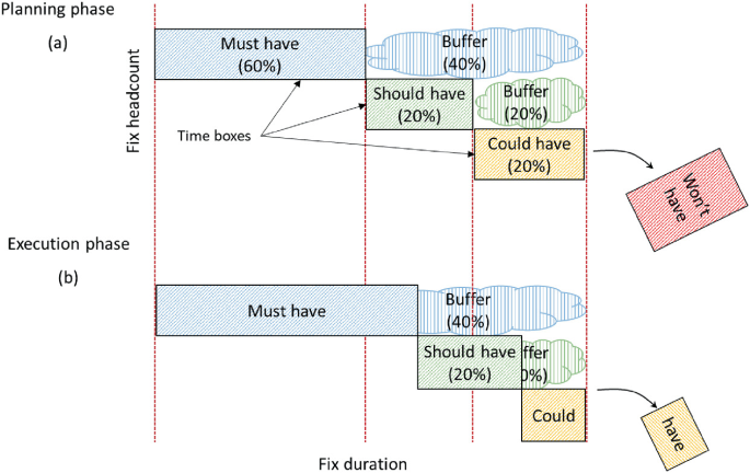
During the project planning phase, see Fig. 1.a, features are allocated to one of four sets: Must Have, Should Have, Could Have, and Won’t Have on the basis of customer preferences and dependencies until the respective budgets are exhausted.

Fig. 1.

MoSCoW rules at play: a) During planning, b) in execution

During execution, Fig. 1.b, features in the Must Have category are developed first, those in the Should Have second, and those in the Could Have, in third place. If at any time the work in any category requires more effort than planned, work on them will continue at the expense of those in the lower preference categories which will be pushed out of scope in the same amount as the extra effort required. The advantage for the project sponsor is that, whatever happens, he or she can rest assured of getting a working product with an agreed subset of the total functionality by the end of the project.

For the MoSCoW method to be accepted by the developer as well as by the sponsor of a project, the risk of partial deliveries must be shared between both of them through incentive contracts since approaches like firm fixed price or time and materials, that offloads most of the risk on only one of the parties could be either, prohibitive or unacceptable to the other. Contractually, the concept of agreed partial deliveries might adopt different forms. For example, the contract could establish a base price for the Must Have set, with increasingly higher bonuses or rewards for the Should Have and Could Have releases. Conversely the contract could propose a price for all deliverables and include penalties or discounts if the lower priority releases are not delivered. This way the incentives and disincentives will prevent the developer from charging a premium price to protect itself from not delivering all features while the sponsor, is assured the developer will do its best, in order to win the rewards.

3 The Monte Carlo Simulation

The Monte Carlo method is a random sampling technique used to calculate probability distributions for aggregated random variables from elementary distributions. The technique is best applied to problems not amenable to closed form solutions derived by algebraic methods.

The Monte Carlo method involves the generation of random samples from known or assumed elementary probability distributions, the aggregation or combination of the sample values according to the logic of the model been simulated and the recording of the calculated values for the purpose of conducting an ex-post statistical analysis.

The technique is widely used [3, 4] in probabilistic cost, schedule and risk assessments and numerous tools³ exist to support the computations needed.

The results presented in the paper were calculated using @Risk 7.5. As these are the product of simulation runs, they might slightly differ from one run to another, or when using a different number of iterations or platforms.

The rest of the section explains the model used to generate the cumulative probability curves and calculate the PoD for each MoSCoW category: Must Have (MH), Should Have (SH) and Could Have (CH), with the purpose of allowing interested readers replicate the studies or develop their own simulations. Those not so inclined might skip it, with little or no loss in understanding the paper. The name of the parameters should make them self-explanatory however, conceptual definitions about its meaning and usage will be provided throughout the paper.

The probability of completing all features in a given category in, or under, an $x$ amount of effort is defined as:

$$ F_{MH} \left( x \right)\,=\,P\left( {EffortRequired_{{MH { }}} \le { }x} \right) $$

$$ F_{SH} \left( x \right)\,=\,P\left( {EffortRequired_{MH} \,{ + }\,{ }EffortRequired_{{SH{ }}} { } \le { }x} \right) $$

$$ F_{CH} \left( x \right)\,=\,P\left( {EffortRequired_{MH} \,{ + }\,EffortRequired{ }_{SH} \,{ + }\,{ }EffortRequired_{CH} { } \le { }x} \right) $$

The cumulative distribution functions: $F_{MH} \left( x \right), \,F_{SH} \left( x \right)\, {\text{and}}\, F_{CH} \left( x \right)$, are built by repeatedly sampling and aggregating the effort required by the features included in each category.

$$ EffortRequired_{MH} \,=\,\sum\nolimits_{{\forall { }i{ } \in{ }MH}} {EffortFeature_{i} } $$

$$ EffortRequired_{SH} \,=\,\sum\nolimits_{{\forall { }j{ } \in { }SH}} {EffortFeature_{j} } $$

$$ EffortRequired_{CH} \,=\,\sum\nolimits_{{\forall { }k{ } \in { }CH}} {EffortFeature_{k} } $$

$$ EffortFeature_{i} = \left\{ {\begin{array}{*{20}l} {{\text{Low confindence estimates: }}RndUniform\left( {Estimate_{i} {, }\,u\, \times \,Estimate_{i} {, }\,r} \right){ }} \hfill \\ {{\text{Typical estimates: }}RndTriangular\left( {{0}{\text{.8}}\, \times \,Estimate_{i} {,}\,{ }Estimate_{i} {, }\,u\, \times \,Estimate_{i} {,}\,{ }r} \right){ }} \hfill \\ \end{array} } \right. $$

similarly, for features j and k, and:

$$ {\text{u = }}\left\{ {\begin{array}{*{20}c} {{1}{\text{.5}}} & {} & {{50}{\% }} \\ {{2}{\text{.0}}} & {\text{underestimation of up to}} & {{100}{\% }} \\ {{3}{\text{.0}}} & {} & {{200}{\% }} \\ \end{array} } \right. $$

$$ {\text{r = }}\left\{ {\begin{array}{*{20}c} {0} & {} & {\text{independent estimates}} \\ {} & {\text{global correlation coefficient for}} & {} \\ {{0}{\text{.6}}} & {} & {\text{correlated estimates}} \\ \end{array} } \right. $$

subject to the maximum allocation of effort for each category:

$$ \sum\nolimits_{{\forall { }i{ } \in { }MH}} {Estimate_{i} { } \le { 0}{\text{.6}}\, \times \,DevelopmentBudget} $$

$$ \sum\nolimits_{{\forall { }j{ } \in { }SH}} {Estimate_{i} { } \le { 0}{\text{.2}}\, \times \,DevelopmentBudget} $$

$$ \sum\nolimits_{{\forall { }i{ } \in { }MH}} {Estimate_{k} { } \le { 0}{\text{.2}}\, \times DevelopmentBudget} $$

The Probability of Delivery (PoD) of each category is defined as:

$$ PoD_{MH} \, = \,F_{MH} \left( {DevelopmentBudget} \right) $$

$$ PoD_{SH} \, = \,F_{SH} \left( {DevelopmentBudget} \right) $$

$$ PoD_{CH} \,=\,F_{CH} \left( {DevelopmentBudget} \right) $$

All quantities are normalized for presentation purposes by dividing them by the $DevelopmentBudget$.

4 Low and Typical Confidence Scenarios

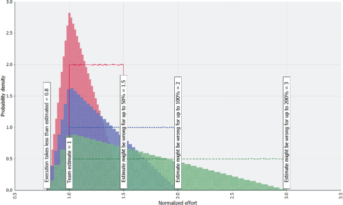
Figure 2 contrasts the two scenarios mentioned in the introduction. The low confidence scenario is characterized by the uniform distribution of the potential efforts required to realize each feature, with the lower limit of each distribution corresponding to the team’s estimated effort for the feature and their upper to increments of 50, 100 and 200% above them, to express increasing levels of uncertainty. Since all values in the interval have equal probability, this scenario corresponds to a maximum uncertainty state [8]. This situation, however unrealistic it might seem, is useful to calculate a worst case for the PoD of each category. In the typical confidence scenario, the potential efforts are characterized by a right skewed triangular distributions, in which the team’s estimates correspond to the most likely value of the distribution, meaning the realization of many features will take about what was estimated, some will take some more and a few could take less.

Fig. 2.

Probability distributions for the effort required by each feature in the low (uniform distributions) and typical (triangular distributions) confidence scenarios

The right skewness of the typical estimate distributions is predicated on our tendency to estimate based on imagining success [9], behaviors like Parkinson’s Law⁴ and the Student Syndrome⁵, which limit the potential for completing development with less effort usage than estimated, and the fact that the number of things that can go wrong is practically unlimited [10, 11]. Although many distributions fit this pattern, e.g. PERT, lognormal, etc., the triangular one was chosen for its simplicity and because its mass is not concentrated around the most likely point [12], thus yielding a more conservative estimate than the other distributions mentioned.

As before, the right extreme of the distribution takes values corresponding to 50, 100 and 200 percent underestimation levels. For the lower limit however, the 80 percent of the most likely value was chosen for the reasons explained above.

Considering this second scenario is important, because although having a worst case for the PoDs is valuable as they tell the lowest the probabilities could be, relying on them for decision making may lead to lost opportunities because of overcautious behaviors.

5 Level of Underestimation, Correlation, Number of Features in a Category, Feature Dominance and Non-traditional Budget Allocations

Before calculating the PoDs for each MoSCoW category under the two scenarios, the impact of different factors on the PoD is explored with the purpose of developing an appreciation for how they affect the results shown, i.e. what makes the PoDs go up or down. Understanding this is important for those wanting to translate the conclusions drawn here to other contexts.

Although the analysis will be conducted only for the low confidence estimates for reasons of space, the same conclusions applies to the typical estimates scenario, with the curves slightly shifted to the left.

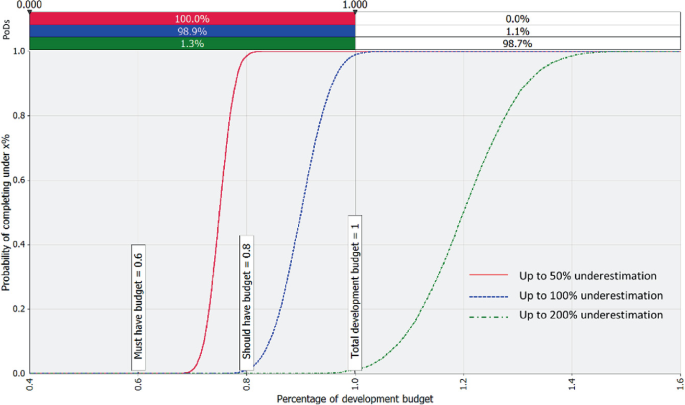
Figure 3 shows the impact of underestimation levels of up to 50, 100 and 200% of the features’ individual estimates on the PoD of a Must Have category comprising 15 equal sized features, whose development efforts are independent from each other.

Independent, as used here, means the efforts required by any two features will not deviate from its estimates conjointly due to a common factor such as the maturity of the technology, the capability of the individual developing it or the consistent over optimism of an estimator. When this occurs, the efforts are correlated rather than independent. Having a common factor does not automatically mean the actual efforts are correlated. For example, a feature could take longer because it includes setting up a new technology, but once this is done, it doesn’t mean other features using the same technology would take longer since the it is already deployed. On the other hand, the use of an immature open source library could affect the testing and debugging of all the features in which it is included.

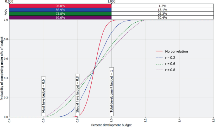
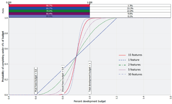
The higher the number of correlated features and the stronger the correlation between them, the more individual features’ efforts would tend to vary in the same direction, either requiring less or more of it, which would translate into higher variability at the total development effort level. This is shown by curves “r = 0.2”, “r = 0.6” and “r = 0.8” in Fig. 4, becoming flatter as the correlation (r) increases.

Correlation brings good and bad news. If things go well, the good auspices will apply to many features, increasing the probability of completing all of them on budget. Conversely, if things do not go as well as envisioned, all affected features will require more effort, and the buffers would not provide enough slack to complete all of them.

Estimating the level of correlation between estimates is not an easy task, it requires assessing the influence one or more common factors could have on the items affected by them, a task harder than producing the effort estimates themselves. So while correlation cannot be ignored at risk of under or over estimating the safety provided by the method, the cost of estimating it, would be prohibitive for most projects. Based on simulation studies, Garvey et al. [13] recommend using a coefficient of correlation of 0.2 across all the estimated elements to solve the dilemma, while Kujawski et al. [14], propose to use a coefficient of 0.6 for elements belonging to the same subsystem, as these would tend to exhibit high commonality since in general, the technology used and the people building it would be the same, and 0.3 for elements on different subsystems, because of the lower commonality.

Fig. 3.

Cumulative completion probabilities under increasing levels of underestimation. The simulation shows a PoD for the Must Have features of 100% for an underestimation level of up to 50%, of 98.9% at up to 100%, and of 1.3% for an underestimation in which each feature can require up to 200% of the estimated budget.

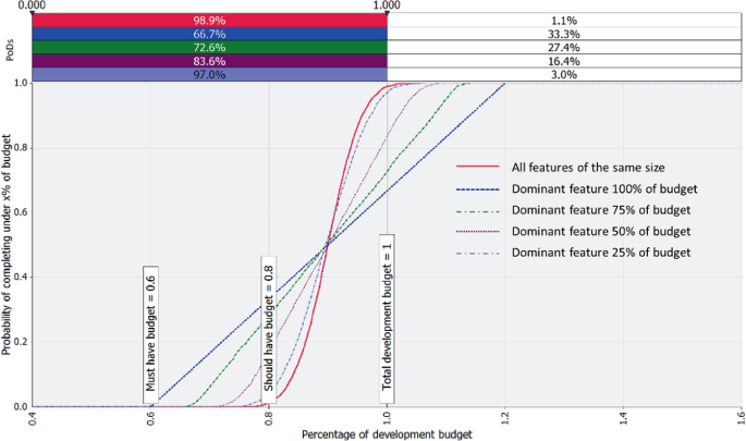
The PoDs are also affected by the number of features in the category as well as by the existence of dominant features, which are features whose realization requires a significative part of the budget allocated to the category. See Figs. 5 and 6.

As in the case of correlation, a small number of features and the presence of dominant features result in an increase in the variability of the estimates. Dominant features, contribute to this increase because it is very unlikely that deviations on their effort requirements could be counterbalanced by the independent deviations of the remaining features in the category. As for the increase of variability with a diminishing number of features, the reason is that with a fewer independent features, the probability of them going all in one direction, is higher than with many features.

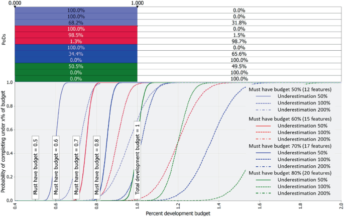
The model in Fig. 7 challenges the premise of allocating 60% of the development budget to the Must Have category and explores alternative assignments of 50, 70 and 80% of the total budget. Reducing the budget allocation from 60 to 50% increases the protection the method affords at the expense of reducing the number of features a team can commit to. Increasing the budget allocation for the Must Have allows developers to promise more, but as will be shown, this is done at the expense of reducing the certainty of delivering it. For the 50% allocation level, there is a 100% chance of delivering the Must Have for underestimations of up to 100%, and of 68.2% for underestimations of up to 200%. At the 70% allocation level, the simulation shows that the PoD for the Must Have, when the possibility of underestimation is up to 50% still is 100%, but that it drops sharply to 34% when the underestimation level rises to up to 100%. For the 80% allocation level, the PoD for the Must Have falls to 49.7% for the up to 50% underestimation level and to 0 for the other two. The rest of the paper will then use the customary 60, 20 & 20% allocation scheme.

Fig. 4.

Probability of completing all features in the Must Have category under a given percent of the budget when the underestimation level is up to 100% and the efforts are correlated (r > 0)

Fig. 5.

Influence of the number of features on the PoD for a Must Have set containing the number of equally sized independent features indicated by the legend on the chart, with an underestimation level of up to 100%. The PoD offered by the method drops sharply when the set contains less than 5 features

Fig. 6.

Influence of a dominant feature on the PoD. Each set, with the exception of the dominant at 100%, contained 15 features, with the dominant feature assigned the bulk of the effort as per the legend in the chart with the remaining budget equally distributed among the other 14 features. The safety offered by the method drops sharply when a feature takes more than 25% of the budgeted effort for the category. Underestimation of up to 100% and independent efforts

Fig. 7.

Probability of delivering all Must Have features for Must Have budget allocations of 50, 60, 70 and 80% under different underestimation conditions. The respective number of Must Have features for each budget allocation were 12, 15, 17, and 20.

6 Probabilities of Delivery for Each MoSCoW Category

This section discusses the PoDs for each MoSCoW category: Must Have, Should Have and Could Have under the following conditions:

• 1. Low confidence estimation, independent efforts

• 2. Low confidence estimation, correlated efforts

• 3. Typical estimation, independent efforts

• 4. Typical estimation, correlated efforts

In all cases, the underestimations considered are of up to 50, 100 and 200% of the estimated effort, a 60/20/20 effort allocation scheme and a Must Have category comprising 15 equal sized features with Should and Could Have categories comprising 5 equal sized features each. These assumptions are consistent with the precedent analysis and with the small criteria in the INVEST [15] list of desirable properties for user stories. For the correlated efforts cases, the article follows Kujaswki’s recommendation, of using an r = 0.6, as many of the attributes of an agile development project: dedicated small teams, exploratory work and refactoring, tend to affect all features equally.

6.1 Low Confidence, Independent Efforts

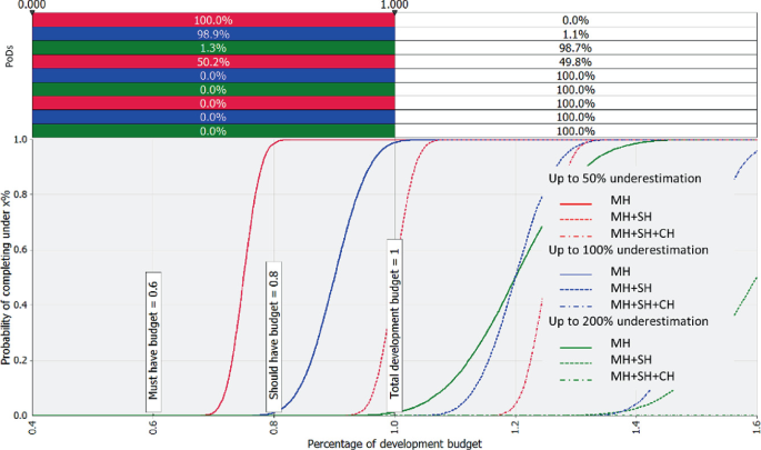
Figure 8 shows the PoDs for all MoSCoW categories for the low confidence, uncorrelated features, r = 0, model. At up to 50% underestimation, the probability of delivering all Must Have is 100%, as expected, and the probability of delivering all Should Have is 50.2%. At up to 100% underestimation, the probability of delivering all the Must Have still high, 98.9% but the probability of completing all the Should Have drops to 0. At up to 200% the probability of delivering all the Must Haves is pretty low, at 1.3%. In no case it was possible to complete the Could Have within budget.

6.2 Low Confidence, Correlated Efforts

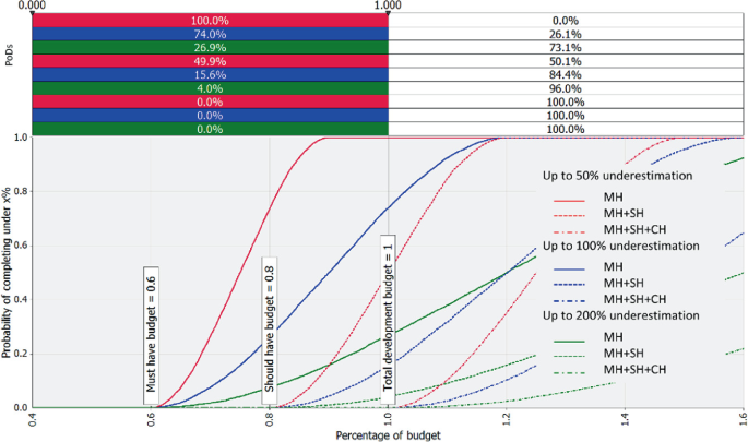
As shown by Fig. 9, in this case the variability of the aggregated efforts increases, with the outermost points of the distribution becoming more extreme as all the efforts tend to move in unison in one or another direction. Comparing the PoDs for this case with those of the previous one, it seems paradoxical, that while the PoD for the Must Have at 100% underestimation level goes down from 98.9 to 74.0, the PoD for the same category at 200% underestimation level goes up from 1.3 to 26.9%! This is what was meant when it was said that correlation brought good and bad news.

Fig. 8.

Probability of delivering all features in a category in the case of low confidence estimates under different levels of underestimation when the efforts required by each feature are independent (r = 0)

To understand what is happening, it suffices to look at Fig. 10. Figure 10.a shows histograms of the Must Have aggregated independent efforts for uncertainty levels of 50, 100 and 200%. Because of the relatively lower upper limit and the tightness of the distribution spread afforded by the sum of independent efforts, the 100% uncertainty distribution fits almost entirely to the left of the total budget, scoring this way a high PoD. A similar argument could be made for the 200% uncertainty level, except that this time, the distribution is almost entirely to the right of the total budget, thus yielding a very low PoD. As could be seen in Fig. 10.b, when the efforts are correlated, the distributions spread more widely, making part of the 100% distribution fall to the right of the total budget line, reducing its PoD, and conversely, part of the 200% distribution might fall to the left of the line, thus increasing its PoD, which is what happened with this particular choice of parameter values.

Fig. 9.

Probability of delivering all features in a category in the case of low confidence estimates under different levels of underestimation when the efforts required by each feature are highly correlated (r = 0.6)

Fig. 10.

Histograms for Must Have features’ effort (a) left – independent efforts, (b) right – correlated efforts

6.3 Typical Estimates

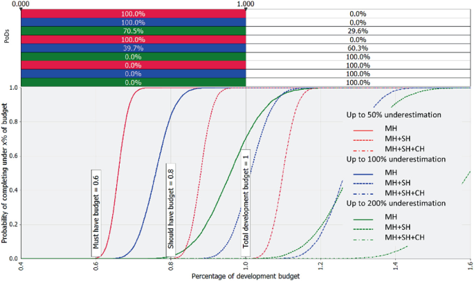
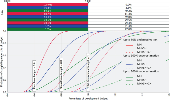
Figures 11 and 12 show the typical estimates’ PoDs for uncorrelated and correlated efforts respectively. As expected, all the PoDs in this scenario are higher than in the case of the low confidence estimates. In the case of independent efforts, at up to 50% underestimation, the PoDs for the Must Have and the Should Have are 100%. At up to 100% underestimation, the PoD for the Must Have is 100% with the PoD for Should Have dropping to 39.7%. At up to 200% the probability of delivering all the Must Haves still high, at 70.5%, but there is no chance of delivering the Should Have. In no case, any Could Have were completed. For the correlated efforts case, the respective probabilities at 50% underestimation are: 100% for the Must Have, 88.7% for the Should Have and 20.6% for the Could Have. At 100% underestimation: 96.4, 50.3 and 8.6% respectively and at 200% underestimation: 59.8, 20.5 and 3%.

Fig. 11.

Probability of delivering all features in a category in the case of typical estimates under different levels of underestimation when the efforts required by each feature are independent (r = 0)

Fig. 12.

Probability of delivering all features in a category in the case of typical estimates under different levels of underestimation when the efforts required by each feature are highly correlated (r = 0.6).

7 Summary

This article sought to quantitatively answer the following questions:

• 1. What are the probabilities of delivering all the features in each of the categories: Must Have, Should Have and Could Have, under varying levels of under and overestimation of the features’ development efforts?

• 2. What is the influence of features’ sizes, feature dominance, number of features, and correlation between development efforts in said probabilities?

• 3. What is the effect of budget allocations other than the customary 60/20/20 on them?

To answer question 1, it is necessary to look at Table 1 which summarizes the results for the low confidence and typical estimates scenarios, for the three levels of underestimation studied: 50, 100 and 200%.

Table 1. PoD summary for the three MoSCoW categories under different conditions

Not surprisingly, the results indicate that the method consistently yields a high PoD for the Must Have features. What is noteworthy, is its resilience in face of up to 100% underestimation of individual features in the category. For the Should Have, the results are robust for up to 50% of underestimation and with regards to the Could Have, they should only be expected if destiny is smiling upon the project.

Question 2 is important for practitioners preparing release plans. For the method to offer these levels of certainty, the number of features included in each category should be at least 5 with none of them requiring more than 25% of the effort allocated to the category. If these conditions are not met, the safety offered by the method drops sharply. Correlation, as mentioned before, is a mixed blessing. Depending on which direction things go, it can bring the only possibility of completing all the features in the project. Notice that in Table 1, all the Could Have can only be completed when the efforts are highly correlated since all of them must be low. Under the independence assumption, when some could be low and others high, there is no chance of completing them on or under budget.

With regards to question 3, the 60, 20, 20% allocation seems to be the “Goldilocks” solution, balancing predictability with level of ambition. As shown by Fig. 7, changing the allocation from 60 to 70%, has a dramatic impact on the safety margin which, at the up to 100% underestimation level, drops from 98.5 to 34%.

Finally, it is worth making clear, that the analysis refers to variations in execution times of planned work and not changes in project scope, which should be addressed differently.

The author gratefully acknowledges the helpful comments of Hakan Erdogmus. Diego Fontdevila and Alejandro Bianchi on earlier versions of this paper.

References

Agile Business Consortium: Chapter 10 MoSCoW Prioritization, January 2014. https://www.agilebusiness.org/page/ProjectFramework_10_MoSCoWPrioritisation. Accessed 10 Oct 2021
Cohn, M.: Agile Estimationg and Planning. Prentice Hall, Upper Saddle River (2006)
Garvey, P.: Elements of Cost Risk Analysis. MITRE Corporation (2014)
Magennis, T.: Managing software development risk using modeling and Monte Carlo simulation. In: Lean Software and Systems Consortium Conference, Boston (2012)
Clegg, D., Baker, R.: CASE Method Fast-track: A RAD Approach. Addison-Wesley, Reading (1994)
Miranda, E.: Planning and Executing Time Bound Projects. IEEE Comput. (2002)
DSDM Consortium: Not longer accessible. http://www.dsdm.org/version4/2/public/default.asp
Shu-Cherng, F., Tsao, H.: Entropy optimization: shannon measure of entropy and its properties. In: Encyclopedia of Optimization, Springer, Boston (2001). https://doi.org/10.1007/0-306-48332-7_119
Newby Clark, I., Buehler, R., Koehler, D., Griffin, D.: People focus on optimistic scenarios and disregard pessimistic scenarios while predicting task completion times. J. Exp. Psychol. Appl. (2000)
Halkjelsvik, T., Jørgensen, M.: Time Predictions: Understanding and Avoiding Unrealism in Project Planning and Everyday Life, Springer, Cham (2018). https://doi.org/10.1007/978-3-319-74953-2
Kitchenham, B., Linkman, S.: Estimates, uncertainty and risk. IEEE Softw. (1997)
Hulett, D.: Practical Schedule Risk Analysis, Gower (2009)
Garvey, P., Book, S.C.R.: Probability Methods for Cost Uncertainty Analysis, 2nd. CRC Press (2016)
Kujawski, E., Edwards, W.R., Alvaro, M.L.: Incorporating psychological influences in probabilistic cost analysis. Syst. Eng. 7(3) (2004)
Wake, B.: INVEST in Good Stories, and SMART Tasks. XP123, 17 8 (2003). https://xp123.com/articles/invest-in-good-stories-and-smart-tasks/. Accessed 19 Nov 2021
Author information
Authors and Affiliations
Corresponding author
Editor information
Editors and Affiliations
Rights and permissions
Open Access This chapter is licensed under the terms of the Creative Commons Attribution 4.0 International License (http://creativecommons.org/licenses/by/4.0/), which permits use, sharing, adaptation, distribution and reproduction in any medium or format, as long as you give appropriate credit to the original author(s) and the source, provide a link to the Creative Commons license and indicate if changes were made.
The images or other third party material in this chapter are included in the chapter's Creative Commons license, unless indicated otherwise in a credit line to the material. If material is not included in the chapter's Creative Commons license and your intended use is not permitted by statutory regulation or exceeds the permitted use, you will need to obtain permission directly from the copyright holder.
Copyright information
© 2022 The Author(s)
About this paper
Cite this paper
Miranda, E. (2022). Moscow Rules: A Quantitative Exposé. In: Stray, V., Stol, KJ., Paasivaara, M., Kruchten, P. (eds) Agile Processes in Software Engineering and Extreme Programming. XP 2022. Lecture Notes in Business Information Processing, vol 445. Springer, Cham. https://doi.org/10.1007/978-3-031-08169-9_2
Download citation
DOI: https://doi.org/10.1007/978-3-031-08169-9_2
Published:
Publisher Name: Springer, Cham
Print ISBN: 978-3-031-08168-2
Online ISBN: 978-3-031-08169-9
eBook Packages: Computer ScienceComputer Science (R0)