
Abstract
English translation of the first chapter of Ernst Schröder’s Lehrbuch der Arithmetik und Algebra für Lehrer und Studirende. Schröder discusses the nature of numbers in general and of the natural numbers in particular, treating numbers as “arbitrary signs created by us for a wide variety of purposes.” His notion that natural numbers “serve as measures of the numerousness of things” leads him to discuss one-to-one correspondences at some length. He also explores the fundamental properties of equality, inequality, and logical subordination (the relation that holds, for example, between a species and its genus). Schröder’s interest in logical topics is evident in his reflections on “general number-signs” or, as we would now say, universally quantified variables.
Access this chapter
Tax calculation will be finalised at checkout
Purchases are for personal use only
Notes
- 1.
[[Numbers in double square brackets give Schröder’s original pagination. Other items in double square brackets are comments by your translator.—Trans.]]
- 2.
- 3.
[[Schröder frequently sets remarks in smaller type than the rest of the main text. The message seems to be that this material is of lesser importance. – Trans.]]
- 4.
For an instructive example of another sort, imagine being required to count the beauties of an artwork. [[At the very end of his book Schröder appended several pages of addenda citing by page and line number the passage on which he was commenting. The foregoing is his first addendum. He introduced his list of addenda as follows. “Though my book was already in the printer’s hands in September of 1872, the compositor’s strike gave me the opportunity to add a few remarks that occurred to me only after the production process had begun. I append them here in the hope of making my book as complete as possible in the time allowed.” – Trans.]]
- 5.
In the word “series” and the kindred words “system,” “group,” etc. the intention of quantitative comparison is less prominent than in the case of the concept “set.” [[This is Schröder’s second addendum. It may be helpful to note that the German word Menge can mean not only “set,” but also “quantity,” “amount,” or “number” (as in “a number of things”).—Trans.]]
- 6.
[[In his Foreword, Schröder describes a series of four volumes. Only the current (first) volume appeared. – Trans.]]
- 7.
I owe to Prof. Hesse this exceptionally accurate and illuminating description of numbers.
- 8.
The volume you are reading was nearly complete when I first saw Ernst Kossak’s pamphlet of last year (Kossak 1872) from whose brief allusions on p. 16 I learned that Weierstrass regularly offers a similar definition of numerical equality in his lectures.
- 9.
[[“y is connected to z through the idea of an uninterrupted permanence” seems to be an exceptionally obscure way to say that y = z or, at least, that we are determined to treat y and z as identical. The point would then be: if x is connected to y and we are determined to treat y and z as identical, then we are obliged to treat x as connected to z.—Trans.]]
- 10.
[[The point seems to be: if there is a pairing of “ones” with “units” and a pairing of those same “units” with other “ones,” then the composition of the two pairings is a pairing of the former “ones” with the latter “ones.” By the way, though one might expect signs to point at what they signify, Schröder’s arrows point the opposite way.—Trans.]]
- 11.
[[A clear statement of this principle appears below in Sect. 1.16.—Trans.]]
- 12.
[[Could Schröder’s point be that a permutation just is a pairing: a bijection from a set to itself? Of course, then, a natural number would be invariant under any permutation of its ones.—Trans.]]
- 13.
[[Yes, Schröder is assuming something very basic: if set A and set B each have exactly one element, then (1) the one element of A can be connected with the one element of B and (2) this leaves no element of either A or B unconnected (that is, no remainder is possible). This is exactly how Schröder uses his principle in the proof below. Here is a picture of the one and only way to connect element a with element b:

According to Schröder, it is also a picture of the one and only way to connect b with a.—Trans.]]
- 14.
[[As rendered here, the first two sentences of this paragraph are logically equivalent. The second sentence is not the converse (Umkehrung) of the first nor do we need to invoke Schröder’s “basic principle” to get from one to the other. Perhaps Schröder intended something like the following: “A univocal connection cannot assign one unit to more than one unit. Applying our basic principle, we obtain the converse: a univocal connection cannot assign more than one unit to a single unit.” Even on this reading, it is hard to see how the basic principle justifies Schröder’s inference. Be that as it may, Schröder’s point is that each of the following pictures represents a connection between a and b, but neither represents a univocal connection.
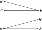
At least, this is what his point must be if the definition below is to be correct.—Trans.]]
- 15.
[[Again, Schröder must mean something like the following. Suppose we are assigning a member of set B to each member of a set A by drawing connecting lines. Member b is assigned to member a if and only if a and b are the endpoints of the same line: the line that connects them. (The basic principle guarantees that a and b are connected by at most one line.) If the assignment is univocal, then each member of A is the endpoint of exactly one line and each member of B is the endpoint of at most one line.—Trans.]]
- 16.
Everyone will, of course, first come to accept this “theorem” on the basis of induction from experience. [[This is an addendum Schröder placed at the end of his book citing the relevant page and line number.—Trans.]]
- 17.
[[Case I:
Case II:
—Trans.]]
- 18.
[[According to Schröder’s basic principle, there is always exactly one way to connect two units. This seems not to imply that there are zero ways to connect one unit with no units—as reasonable as that proposition might be.—Trans.]]
- 19.
Strictly speaking, this proposition is based on an assumption (silently introduced in Sect. 1.16)—namely that the value of each expression and the result of each computation depends only on the meaning (the value) of the operands connected therein, not on their origin or the notation we use to denote them. In view of this and in accordance with the remarks in Sect. 1.16, it really seems more correct to confirm the proposition (and thereby the interchangeability of equal numbers) individually for each of the operations to be introduced later. In the case of addition, we will have to appeal to a general psychological fact (or experience):
If a = α and b = β, then we can assign the ones of a to the ones of α univocally and without remainder. Likewise the ones of b and β. The fact mentioned above is that this assignment persists both in our minds and before our eyes during and after our union of the ones of a and b in the sum a + b and of the ones of α and β in the sum α + β (cf. Sect. 2.1). It follows that a + b = α + β, as desired.
For multiplication, etc., we obtain the proposition as a special case of the above proposition about addition extended to sums with several terms. As for the inverse operations, see Sect. 3.11. [[The foregoing is an addendum Schröder placed at the end of his book citing the relevant passage.—Trans.]]
- 20.
[[One of Cauchy’s own examples is: \(((a))^{\frac {1}{2}}=\pm a^{\frac {1}{2}}\). Schöder himself adds just one pair of parentheses. – Trans.]]
- 21.
[[Our symbols ‘€’ and ‘’ do not quite match Schröder’s notation. His symbols look more like ‘
 ’ and ‘
 ’ .—Trans.]]
 - 22.
[[The illustration Schröder has in mind is:
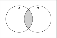
—Trans.]]
- 23.
[[Schröder has ‘major’ and ‘minor’ mixed up here, though he gets it right in the very next sentence.—Trans.]]
- 24.
[[What is generally impermissible is, presumably, replacing the subject with a superordinate concept and the predicate with a subordinate one.—Trans.]]
- 25.
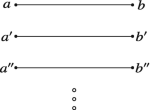
[[Schröder could have written:
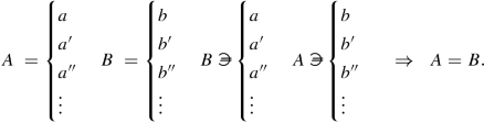
Nowadays we would say:
$$\displaystyle \begin{aligned}A=\{a,a',a'',\ldots\}\subseteq B\;\;\text{and}\;\;B=\{b,b',b'',\ldots\}\subseteq A\;\;\Rightarrow\;\;A=B.\end{aligned}$$—Trans.]]
- 26.
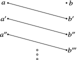
[[Here is a much more literal rendering: “From the joint satisfaction of the propositions

for a series of individual values a, a′, a″, … we can always infer

provided that those values are the only ones admitted by the expression A; provided that, therefore, the second proposition holds for all those individual values, designated by a, that could possibly satisfy the first.”—Trans.]]
- 27.
[[Puzzling. Just a few paragraphs ago, Schröder noted the limitations on substitutions of the latter sort.—Trans.]]
- 28.
[[Yet another use for the symbol ‘ ’. We might say: a maps to b. An Abbildung in mathematics is a mapping.—Trans.]]
- 29.
[[Schröder actually writes: ‘5.6’. Here and in what follows I use the modern notation.—Trans.]]
- 30.
[[As noted above, Schröder’s projected third volume never appeared. –Trans.]]
- 31.
For example, in the well-known textbook by Baltzer . [[Schröder is probably referring to Baltzer (1868). See p. 66 of that work. – Trans.]]
- 32.
[[I am using ‘relation’ to translate Schröder’s ‘Relation’ even though talk of true or false relations may be jarring. – Trans.]]
- 33.
It may be useful to provide an overview in tabular form of the various ways of classifying numbers and equations.
To classify numbers in terms of their notation we might offer the scheme:
$$\displaystyle \begin{aligned} \text{Number-signs:} \begin{cases} \text{Numerical:} \begin{cases} \text{Simple (numerals): e.g.,}\; 5 \\ \text{Compound: e.g.,}\;12-3 \end{cases} \\ \text{Literal:} \begin{cases} \text{Simple: e.g.,}\;a \\ \text{Complex (algebraic expressions): e.g.,}\;5a+1,\;xy,\;a_n. \end{cases} \end{cases} \end{aligned}$$We might say: each number-sign is either “numerical” (built up solely out of numerals) or “literal” (containing at least one letter); furthermore, each of these two kinds of number-sign is subdivided into the “simple” and the “compound.”
As for number-signs such as x + 5 − x or \(\frac {5x}{x}\) in which the letters cancel out under the rules of general arithmetic, there may be some doubt whether they should be classified as numerical or literal. The former is permissible only if we always take those rules for granted.
Compositional structure (complexity) could replace alphabetic character (of a number-sign or its components) as the supreme principle for classifying number-signs.
If we assume the classifications above, the following schemes can be readily understood.
We can classify number-signs in terms of their range of denotation [[nach ihrer Deutigkeit]] (although this will be of importance only for more advanced students):
$$\displaystyle \begin{aligned} \text{Expressions:} \begin{cases} \text{Meaningless }[[{sinnlos}]] \\ \text{Univocal }[[{eindeutig}]]: \\ \text{Ambiguous }[[{mehrdeutig}]] \end{cases} \end{aligned}$$A meaningless expression is non-denoting [[undeutig]]. Speaking very loosely, it represents a non-existent or, we might say, “impossible” number: for example, x when understood to be the number that exceeds itself by 1 (the number satisfying the equation x + 1 = x). Or: “the decimal system digit that exceeds 5 by 8.” Or: “the natural number 2 − 5.” And so on. Only a univocal number-sign represents a number unambiguously [[unzweideutig]]. An ambiguous number-sign encompasses several, indeed a whole class of numbers all at once. For example, \((\sqrt {9})=\pm 3\). Or: the expression that denotes all the “roots” of the equation
$$\displaystyle \begin{aligned}x(x^2+11)=6(x^2+1)\end{aligned}$$would have to subsume the values 1, 2, and 3.
We might classify numbers in terms of their determinacy as follows.
$$\displaystyle \begin{aligned} \text{Numbers:} \begin{cases} \text{Definite:} \begin{cases} \text{Known} \\ \text{Unknown} \end{cases} \\ \text{Indefinite} \end{cases} \end{aligned}$$A known or given definite number is usually numerical (e.g., 1873), but is sometimes literal (e.g., e, π). An unknown or desired definite number is often literal and is determined by an equation (as with x in 2x + 1 = 9 or x(xx − 1) = 60); on the other hand, such a number is often determined by an appellation describing it as the cardinality or measure of some objects. A number can be partly or fully indefinite and, so, “arbitrary” or “general”; such a number is occasionally numerical \(\left (\frac {0}{0}\right )\), but usually literal (as with a and b in the equation a + b − b = a or x in the equation \(x=\frac {x+1}{2}+\frac {x-1}{2}\)).
We can treat a compound numerical expression as known before we have computed it as long as that computation presents no insuperable difficulties.
The difference between an indefinite number and an ambiguous number-sign is that we must keep all the values of an ambiguous number-sign constantly in mind, whereas our understanding of an indefinite number is always univocal whether we think of the number as somehow arbitrary or contemplate the possibility of its full determination. Practice will make this rather subtle distinction entirely clear.
In a given number-domain, we can classify equations as follows.
$$\displaystyle \begin{aligned} \text{Equations:} \begin{cases} \text{Numerical:} \begin{cases} \text{Correct} \\ \text{Incorrect} \end{cases} \\ \text{Literal:} \begin{cases} \text{Analytic} \\ \text{Synthetic} \end{cases} \\ \end{cases} \end{aligned}$$A numerical equation contains no literal numbers, while a literal equation contains at least one. A correct or true numerical equation will be implicit in the rules of general arithmetic; it will “agree” with those rules; e.g., 2 + 3 = 5. An incorrect or false numerical equation will “conflict” with the rules; e.g., 2 + 3 = 7. An analytic literal equation (a “formula”) is unconditionally correct for all values or value-systems of the literal numbers; e.g., a(b + c) = ab + ac, \(x=\frac {x+1}{2}+\frac {x-1}{2}\). A synthetic literal equation is not satisfied by all values (or value-systems) of the literal numbers but only (unconditionally) by some or, indeed, by none; e.g., (a + b)2 = a 2 + b 2, 2x + 1 = 9, x + 1 = x + 2.
In this classification, literal numbers that have a conventionally determined numerical meaning (such as π, etc.) are to be treated as numerical.
It should be pointed out early on that accumulating synthetic equations is easy, but crafting formulas is an art that requires familiarity with the laws of algebraic operations. [[This lengthy note is an addendum Schröder placed at the end of his book citing Sects. 1.25 and 1.26.—Trans.]]
- 34.
Conflating these concepts is an error that Liersemann (for one) recently committed in Liersemann (1871).
- 35.
This point could be disputed. If, instead of a single function-value, we associate a whole system of function-values with each system of argument-values [those systems of function-values varying in size and, so, not forming a system of functions in the usual sense], the result would certainly be a more general concept that may or may not deserve the name “function.”
Although researchers in complex analysis discuss “many-valued” functions, this is just a term of art used to designate a certain class of functions (that are made univocal by decomposing the domain into layers in a well-known way).
I would recommend, when dealing with either functions or numbers, that we treat ambiguity as a property not of the things themselves but only of the expressions we use to denote them. After all, it is quite generally the case that ambivalence and indefiniteness cannot inhere in the things themselves but only in the verbal expression of our ideas of them. It’s bad enough that we follow the familiar practice of describing some operations as “ambiguous” even though, strictly speaking, this is improper. [[This is an addendum Schröder placed at the end of his book citing the relevant page and line number. Your translator never did figure out what the comment in square brackets (von veränderlicher Anzahl, also nicht gerade ein System von Functionen im gewöhnlichen Sinne bildend) is supposed to mean and, so, is not confident about his translation of it. – Trans.]]
- 36.
Our use of symbols to designate functions is analogous to our use of letters to designate numbers. In brief, we use a letter such as f to designate a function that, at the outset, is indeed arbitrary but, once fixed, remains the same function throughout our analysis. [[This is an addendum Schröder placed at the end of his book citing the relevant page.—Trans.]]


 ’ and ‘
 ’ .—Trans.]]


References
Baltzer, R. (1868). Die Elemente der Mathematik (Vol. 1). Leipzig: G. Hirzel.
Cauchy, A. (1821). Cours d’Analyse de l’École Royale Polytechnique. Paris: Debure.
Kossak, E. (1872). Die elemente der Arithmetik. Berlin: Nicolaische Verlagsbuchhandlung.
Kummer, E. E. (1847). Zur Theorie der complexen Zahlen. Journal für die reine und angewandte Mathematik, 35, 319–326.
Liersemann, K. H. (1871). Lehrbuch der Arithmetik und Algebra. Leipzig: Teubner.
Müller, J. H. T. (1855) Lehrbuch der allgemeinen Arithmetik für höhere Lehranstalten. Halle: Verlag der Buchhandlung des Waisenhauses.
Riemann, B. (1867). Über die Hypothesen, welche der Geometrie zu Grunde liegen. Abhandlungen der Königlichen Gesellschaft der Wissenschaften zu Göttingen, 13, 133–152.
Thomae, J. (1870). Abriss einer Theorie der complexen Functionen und der Thetafunctionen einer Veränderlichen. Halle: Louis Nebert.
Author information
Authors and Affiliations
Editor information
Editors and Affiliations
Rights and permissions
Copyright information
© 2022 The Author(s), under exclusive license to Springer Nature Switzerland AG
About this chapter

Cite this chapter
Pollard, S. (2022). Numbers. In: Pollard, S. (eds) Ernst Schröder on Algebra and Logic . Synthese Library, vol 465. Springer, Cham. https://doi.org/10.1007/978-3-031-05671-0_1
Download citation
DOI: https://doi.org/10.1007/978-3-031-05671-0_1
Published:
Publisher Name: Springer, Cham
Print ISBN: 978-3-031-05670-3
Online ISBN: 978-3-031-05671-0
eBook Packages: Religion and PhilosophyPhilosophy and Religion (R0)