Synthetic Datasets and Evaluation Tools for Inductive Neural Reasoning

Abstract

Logical rules are a popular knowledge representation language in many domains. Recently, neural networks have been proposed to support the complex rule induction process. However, we argue that existing datasets and evaluation approaches are lacking in various dimensions; for example, different kinds of rules or dependencies between rules are neglected. Moreover, for the development of neural approaches, we need large amounts of data to learn from and adequate, approximate evaluation measures. In this paper, we provide a tool for generating diverse datasets and for evaluating neural rule learning systems, including novel performance metrics.

C. Cornelio and V. Thost: Equal contribution. The work was partly conducted while C.C. was at IBM Research.

Appendices

A Additional Preliminaries

Our measures are based on the concepts of Herbrand base and structure. Generally formal logic distinguishes between syntax (symbols) and its interpretation. Herbrand structures, which are used for interpretation, are however defined solely by the syntactical properties of the vocabulary. The idea is to directly take the symbols of terms as their interpretations which, for example, has proven useful in the analysis of logic programming.

The focus is on ground terms (e.g., atoms and rules), which are terms that do not contain variables.

The Herbrand base of a FOL vocabulary (of constants, predicates, etc.) is the set of all ground terms that can be formulated in the vocabulary. If the vocabulary does not contain constants, then the language is extended by adding an arbitrary new constant.

A Herbrand model interprets terms over a Herbrand base, hence it can be seen as a set of ground atoms. Let T be the set of all variable-free terms over a vocabulary V. A structure S over V and with base U is said to be a Herbrand structure iff $U=T_0$ and $c^S$ = c for every constant $c\in V$.¹³

B Dataset Generation

In this section, we describe the generation process of the rules and facts in detail, assuming the generator parameters (also configuration) listed in Sect. 3 to be set.

Preprocessing. As already mentioned, most parameters are determined randomly in a preprocessing step if they are not fixed in the configuration, such as the symbols that will be used, the numbers of DGs to be generated, and their depths. However, all random selections are within the bounds given in the configuration under consideration; for instance, we ensure that the symbols chosen suffice to generate rule graphs and fact sets of selected size and that at least one graph is of the given maximal depth.

Rule Generation. According to the rule set category specified and graph depths determined, rules (nodes in the graphs) of form (2) are generated top down breadth first, for each of the rule graphs to be constructed. The generation is largely at random, that is, w.r.t. the number of child nodes of a node and which body atom they relate to; the number of atoms in a rule; and the predicates within the latter, including the choice of the target predicate (i.e., the predicate in the head of the root) in the very first step. RuDaS also offers the option that all graphs have the same target predicate. To allow for more derivations, we currently only consider variables as terms in head atoms; the choice of the remaining terms is based on probabilities as described in the following. Given the atoms to be considered (in terms of their number and predicates) and an arbitrary choice of head variables, we first determine a position for each of the latter in the former. Then we populate the other positions one after the other: a head variable is chosen with probability $p_h=\frac{1}{5}$; for one of the variables introduced so far, we have probability $p_v=(1-p_h) * \frac{3}{4}$; for a constant, $p_c=(1-p_h) * (1-p_v) * \frac{1}{10}$; and, for a fresh variable, $p_f=(1-p_h) * (1-p_v) * (1-p_c)$. While this conditional scheme might seem rather complex, we found that it works best in terms of the variety it yields; also, these probabilities can be changed easily.

Fact Generation. The fact generation is done in three phases: we first construct a set $\mathbb {D}$ of relevant facts in a closed-world setting, consisting of support facts $\mathbb {S}$ and their consequences $\mathbb {C}$, and then adapt it according to $n_{\text {OW}}$ and $n_{\text {Noise*}}$.

As it is the (natural) idea, we generate facts by instantiating the rule graphs multiple times, based on the assumption that rule learning systems need positive examples for a rule to learn that rule, and stop the generation when the requested number of facts has been generated. We actually stop later because we need to account for the fact that we subsequently will delete some of them according to $n_{\text {OW}}$. More specifically, we continuously iterate over all rule graphs, for each, select an arbitrary but fresh variable assignment $\sigma$, and then iterate over the graph nodes as described in the following, in a bottom-up way. First, we consider each leaf n and corresponding rule of form (2) and generate support facts $\sigma (\alpha _1),\dots ,\sigma (\alpha _m)$. Then, we infer the consequences based on the rules and all facts generated so far. For every node n on the next level and corresponding rule of form (2), we only generate those of the facts $\sigma (\alpha _1),\dots ,\sigma (\alpha _m)$ as support facts which are not among the consequences inferred previously. We then again apply inference, possibly obtaining new consequences, and continue iterating over all nodes in the graph in this way. We further diversify the process based on two integer parameters, $n_{\text {DG}}$ and $n_{\text {Skip}}$: in every $n_{\text {DG}}$-th iteration the graph is instantiated exactly in the way described; in the other iterations, we skip the instantiation of a node with probability 1/$n_{\text {Skip}}$ and, in the case of DR-DGs, only instantiate a single branch below disjunctive nodes. We implemented this diversification to have more variability in the supports facts, avoiding to have only complete paths from the leaves to the root.

In the open-world setting, we subsequently construct a set $\mathbb {D} _{\text {OW}}$ by randomly deleting consequences from $\mathbb {D}$ according to the open-world degree given: assuming $\mathbb {T} \subseteq \mathbb {C}$ to be the set of target facts (i.e., consequences containing the target predicate), we remove $n_{\text {OW}} \%$ from $\mathbb {C} \setminus \mathbb {T}$, and similarly $n_{\text {OW}} \%$ from $\mathbb {T}$. In this way, we ensure that the open-world degree is reflected in the target facts. Though, there is the option to have it more arbitrary by removing $n_{\text {OW}} \%$ from $\mathbb {C}$ instead of splitting the deletion into two parts.

The noise generation is split similarly. Specifically, we construct a set $\mathbb {D} _{\text {OW+Noise}}$ based on $\mathbb {D} _{\text {OW}}$ by arbitrarily removing $n_{\text {Noise-}} \%$ from $\mathbb {S}$, and by adding arbitrary fresh facts that are neither in $\mathbb {C}$ (i.e., we do not add facts we have removed in the previous step) nor contain the target predicate such that $\mathbb {D} _{\text {OW+Noise}} \setminus \mathbb {T}$ contains $n_{\text {Noise+}} \%$ of noise. In addition, we add arbitrary fresh facts on the target predicate that are not in $\mathbb {T}$ already such that subset of $\mathbb {D} _{\text {OW+Noise}}$ on that predicate finally contains $n_{\text {Noise+}} \%$ of noise.

Output. The dataset generation produces: the rules; a training set ($\mathbb {D} _{\text {OW+Noise}}$), which is of the requested size, and fulfills $n_{\text {OW}}$, $n_{\text {Noise+}}$, and $n_{\text {Noise-}}$; and custom fact sets $\mathbb {S} '$ and $\mathbb {C} '$ for our evaluation tools generated in the same way as $\mathbb {S}$ and $\mathbb {C}$. For further experiments, RuDaS also outputs $\mathbb {D}$, $\mathbb {D} _{\text {Noise}}$ (an adaptation of $\mathbb {D}$ which contains noise but all of $\mathbb {C}$), $\mathbb {D} _{\text {OW}}$, $\mathbb {S}$, and $\mathbb {C}$ (see also the end of Sect. C).

Table 5. Overview of our generated datasets, altogether 196; column # is the count of datasets described in the corresponding row. All other numbers are averages. For Chain, we have $n_{\text {OW}} =0.3$, $n_{\text {Noise-}} =0.2$, and $n_{\text {Noise+}} =0.1$. For RDG and DRDG: $n_{\text {OW}} \in \{0.2,0.3,0.4\}$, $n_{\text {Noise-}} \in \{0.15,0.2,0.3\}$, and $n_{\text {Noise+}} \in \{0.1,0.2,0.3\}$. Note that the size bounds of our fact sets are not strict, some sizes are slightly larger than expected (e.g., 1065 for size M) because our initial generation needs to take into account that some facts, e.g., consequences, may be removed thereafter.

C Statistics of RuDaS .v0

Table 5 provides statistics regarding RuDaS .v0: the generated set of datasets available to the community in our repository.

D Approaches to Rule Learning

Classical ILP systems such as FOIL [24] and Progol [19] usually apply exhaustive algorithms to mine rules for the given data and either require false facts as counter-examples or assume a closed world (for an overview of classical ILP systems see Table 2 in [32]). The closed-world assumption (CWA) (vs. open world assumption or OWA) states that all facts that are not explicitly given as true are assumed to be false.

Today, however, knowledge graphs with their often incomplete, noisy, heterogeneous, and, especially, large amounts of data raise new problems and require new solutions. For instance, real data most often only partially satisfies the CWA and does not contain counter-examples. Moreover, in an open world, absent facts cannot be considered as counter-examples either, since they are not regarded as false. Therefore, successor systems, with AMIE+ [12] and RDF2Rules [34] as the most prominent representatives, assume the data to be only partially complete and focus on rule learning in the sense of mining patterns that occur frequently in the data. Furthermore, they implement advanced optimization approaches that make them applicable in wider scenarios. In this way, they address already many of the issues that arise with today’s knowledge graphs, still maintaining their processing exhaustive.

Recently, neural rule learning approaches have been proposed: [4, 10, 17, 22, 27, 35]. These methodologies seem a promising alternative considering that deep learning copes with vast amounts of noisy and heterogeneous data. The proposed solutions consider vector or matrix embeddings of symbols, facts and/or rules, and model inference using differentiable operations such as vector addition and matrix composition. However, they are still premature: they only learn certain kinds of rules or lack scalability (e.g., searching the entire rule space) and hence cannot compete with established rule mining systems such as AMIE+ yet, as shown in [22], for example.

E System Configurations

All the systems have the same computational restrictions (i.e. CPU, memory, time limit, etc.). The reader can find all the details (scripts etc.) in the RuDaS GitHub repository.

FOIL

• Paper: Learning logical definitions from relations. Machine Learning, 5:239-266, 1990.

  https://www.semanticscholar.org/paper/Learning-logical-definitions-from-relations-Quinlan/554f3b32b956035fbfabba730c6f0300d6955dce

• Source Code:

  http://www.rulequest.com/Personal/ or

  http://www.cs.cmu.edu/afs/cs/project/ai-repository/ai/areas/learning/systems/foil/foil6/0.html, Version: 6

• Running configuration:

  

  -m 200000: used when the max tuples are exceeded

• Parameter for accepting the rules: NA – all the rules are accepted

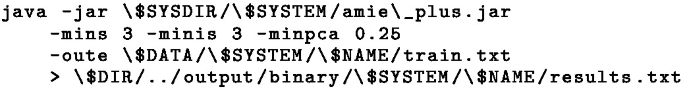
Amie+

• Paper: Fast Rule Mining in Ontological Knowledge Bases with AMIE+. Luis Galárraga, Christina Teflioudi, Fabian Suchanek, Katja Hose. VLDB Journal 2015. https://suchanek.name/work/publications/vldbj2015.pdf

• Source Code:

  https://www.mpi-inf.mpg.de/departments/databases-and-information-systems/research/yago-naga/amie/, Version of 2015-08-26

• Running configuration:

  

• Parameter for accepting the rules: learned using grid-search $=0.7$ – all the rules with PCA Confidence $> 0.7$ are accepted

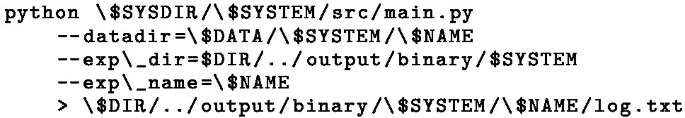
Neural-LP

• Paper: Differentiable Learning of Logical Rules for Knowledge Base Reasoning.Fan Yang, Zhilin Yang, William W. Cohen. NIPS 2017. https://arxiv.org/abs/1702.08367

• Source Code:

  https://github.com/fanyangxyz/Neural-LP

• Running configuration:

  

• Parameter for accepting the rules: learned using grid-search $=0.6$ – all the rules with ri-normalized prob $> 0.6$ are accepted

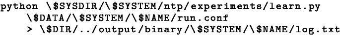
Neural-theorem prover (ntp)

• Paper: End-to-end Differentiable Proving. Tim Rocktaeschel and Sebastian Riedel. NIPS 2017. http://papers.nips.cc/paper/6969-end-to-end-differentiable-proving

• Source Code:

  https://github.com/uclmr/ntp

• Running configuration:

  

• Parameter for accepting the rules: learned using grid-search $=0.0$ – all the rules are accepted

References

Alexe, B., Tan, W.C., Velegrakis, Y.: Stbenchmark: towards a benchmark for mapping systems. Proc. VLDB Endow. 1(1), 230–244 (2008)
Arocena, P.C., Glavic, B., Ciucanu, R., Miller, R.J.: The ibench integration metadata generator. Proc. VLDB Endow. 9(3) (2015)
Benedikt, M., et al.: Benchmarking the chase. In: Proceedings of PODS. ACM, pp. 37–52 (2017)
Campero, A., Pareja, A., Klinger, T., Tenenbaum, J., Riedel, S.: Logical rule induction and theory learning using neural theorem proving. CoRR abs/1809.02193 (2018)
Ceri, S., Gottlob, G., Tanca, L.: What you always wanted to know about datalog (and never dared to ask). In: IEEE Trans. on Knowl. and Data Eng. 1(1), 146–166 (1989)
Dong, H., Mao, J., Lin, T., Wang, C., Li, L., Zhou, D.: Neural logic machines. In: Proceedings of ICLR (2019)
Dong, X.L., et al.: Knowledge vault: A web-scale approach to probabilistic knowledge fusion. In: Proceedings of KDD, pp. 601–610 (2014)
Estruch, V., Ferri, C., Hernández-Orallo, J., Ramírez-Quintana, M.J.: Distance based generalisation. In: Kramer, S., Pfahringer, B. (eds.) ILP 2005. LNCS (LNAI), vol. 3625, pp. 87–102. Springer, Heidelberg (2005). https://doi.org/10.1007/11536314_6
Estruch, V., Ferri, C., Hernández-Orallo, J., Ramírez-Quintana, M.J.: An integrated distance for atoms. In: Blume, M., Kobayashi, N., Vidal, G. (eds.) FLOPS 2010. LNCS, vol. 6009, pp. 150–164. Springer, Heidelberg (2010). https://doi.org/10.1007/978-3-642-12251-4_12
Evans, R., Grefenstette, E.: Learning explanatory rules from noisy data. J. Artif. Intell. Res. 61, 1–64 (2018)
Fürnkranz, J., Gamberger, D., Lavrac, N.: Foundations of Rule Learning. Springer, Cognitive Technologies (2012)
Galárraga, L., Teflioudi, C., Hose, K., Suchanek, F.M.: Fast rule mining in ontological knowledge bases with AMIE+. VLDB J. 24(6), 707–730 (2015), code available at https://www.mpi-inf.mpg.de/departments/databases-and-information-systems/research/yago-naga/amie/
Ho, V.T., Stepanova, D., Gad-Elrab, M.H., Kharlamov, E., Weikum, G.: Rule learning from knowledge graphs guided by embedding models. In: Vrandečić, D., et al. (eds.) ISWC 2018. LNCS, vol. 11136, pp. 72–90. Springer, Cham (2018). https://doi.org/10.1007/978-3-030-00671-6_5
ILP: ILP Applications and Datasets. https://www.doc.ic.ac.uk/~shm/applications.html (year na). Accessed 09 Mar 2020
de Jong, M., Sha, F.: Neural theorem provers do not learn rules without exploration. ArXiv abs/1906.06805 (2019)
Krishnan, A.: Making search easier (2018). https://blog.aboutamazon.com/innovation/making-search-easier. Accessed 03 Sept 2020
Minervini, P., Bosnjak, M., Rocktäschel, T., Riedel, S.: Towards neural theorem proving at scale. In: Proceedings of NAMPI (2018)
Minervini, P., Bošnjak, M., Rocktäschel, T., Riedel, S., Grefenstette, E.: Differentiable reasoning on large knowledge bases and natural language. In: Proceedings of AAAI Conference on Artificial Intelligence, vol. 34, no. 04, pp. 5182–5190 (2020)
Muggleton, S.: Inverse entailment and progol. New Gen. Comput. 13(3&4), 245–286 (1995)
Nienhuys-Cheng, S., de Wolf, R.: Foundations of Inductive Logic Programming, vol. 1228. Springer (1997)
Nienhuys-Cheng, S.-H.: Distance between herbrand interpretations: a measure for approximations to a target concept. In: Lavrač, N., Džeroski, S. (eds.) ILP 1997. LNCS, vol. 1297, pp. 213–226. Springer, Heidelberg (1997). https://doi.org/10.1007/3540635149_50
Omran, P.G., Wang, K., Wang, Z.: Scalable rule learning via learning representation. In: Proceedings of IJCAI, pp. 2149–2155 (2018)
Preda, M.: Metrics for sets of atoms and logic programs. Ann. Univ. Craiova 33, 67–78 (2006)
Quinlan, J.R.: Learning logical definitions from relations. Mach. Learn. 5, 239–266 (1990). code available at http://www.cs.cmu.edu/afs/cs/project/ai-repository/ai/areas/learning/systems/foil/foil6/0.html
Raedt, L.D.: Logical and Relational Learning. Springer, Cognitive Technologies (2008)
Ren, H., Hu, W., Leskovec, J.: Query2box: reasoning over knowledge graphs in vector space using box embeddings. In: Proceedings of ICLR (2020)
Rocktäschel, T., Riedel, S.: End-to-end differentiable proving. In: Proceedings of NeurIPS, pp. 3791–3803 (2017). code available at https://github.com/uclmr/ntp
Russell, S., Norvig, P.: Artificial Intelligence: A Modern Approach. Prentice Hall Press (2002)
Seda, A.K., Lane, M.: On continuous models of computation: towards computing the distance between (logic) programs. In: Proceedings of IWFM (2003)
Sinha, K., Sodhani, S., Pineau, J., Hamilton, W.L.: Evaluating logical generalization in graph neural networks. ArXiv abs/2003.06560 (2020)
Sinha, K., Sodhani, S., Pineau, J., Hamilton, W.L.: Evaluating logical generalization in graph neural networks (2020)
Stepanova, D., Gad-Elrab, M.H., Ho, V.T.: Rule induction and reasoning over knowledge graphs. In: d’Amato, C., Theobald, M. (eds.) Reasoning Web 2018. LNCS, vol. 11078, pp. 142–172. Springer, Cham (2018). https://doi.org/10.1007/978-3-030-00338-8_6
Vaclav Zeman, T.K., Svátek, V.: Rdfrules: Making RDF rule mining easier and even more efficient. Semant-Web-J. 12(4), 569–602 (2019)
Wang, Z., Li, J.: Rdf2rules: Learning rules from RDF knowledge bases by mining frequent predicate cycles. CoRR abs/1512.07734 (2015)
Yang, F., Yang, Z., Cohen, W.W.: Differentiable learning of logical rules for knowledge base reasoning. In: Proc. of NeurIPS, pp. 2316–2325 (2017). https://github.com/fanyangxyz/Neural-LP
Yang, Y., Song, L.: Learn to explain efficiently via neural logic inductive learning. In: Proceedings of ICLR (2020)
Author information
Authors and Affiliations
Corresponding author
Editor information
Editors and Affiliations