On the Origin of the Universe: Chaos or Cosmos?

Abstract

I would like to consider the Universe according to the standard Big Bang model, including various quantum models of its origin. In addition, using the theory of nonlinear dynamics, deterministic chaos, fractals, and multifractals I have proposed a new hypothesis, Macek (The Origin of the World: Cosmos or Chaos? Cardinal Stefan Wyszyński University (UKSW) Scientific Editions, 2020). Namely, I have argued that a simple but possibly nonlinear law is important for the creation of the Cosmos at the extremely small Planck scale at which space and time originated. It is shown that by looking for order and harmony in the complex real world these modern studies give new insight into the most important philosophical issues beyond classical ontological principles, e.g., by providing a deeper understanding of the age-old philosophical dilemma (Leibniz, 1714): why does something exist instead of nothing? We also argue that this exciting question is a philosophical basis of matters that influence the meaning of human life in the vast Universe.

Chaos is the score on which reality is written.

Henry Miller (1891–1980)

1 Introduction

In science the evolution the Universe is based on the Big Bang model, which has now become a standard scenario. However, very little is known about the early stages of this evolution, where we should rely on some models, because the required quantum gravity theory is still missing. On the other hand, creation of the Universe is usually an important issue of philosophy. Hence, one should return to great philosophers starting from the Greeks asking the questions about the origin of existence of the world [7], including

• Plato’s creation: a Demiurg transformed an initial chaotic stuff

  into the ordered Cosmos.

• Aristotle’s universe is eternal: the world always existed,

  but needed the possibly atemporal Prime Mover or the First Cause.

In this paper, we would like to consider the origin of the Universe in view of the modern science, including quantum models of creation, and the recent theory of nonlinear dynamics, deterministic chaos, and fractals, see [12]. We hope that these modern studies give also new insight into the most important philosophical issues exceeding the classical ontological principles, e.g., providing a deeper understanding of the age-old philosophical question:

Why does something exist instead of nothing?

Gottfried Wilhelm von Leibniz (1646–1716)

2 The Universe in Modern Science

Here we discuss the Standard Model of the Evolution of the Universe based on the Standard Model of Forces together with selected models of the creation of the world based on quantum theory and modern mathematics [12, ch. 2].

A veritable revolution in understanding of the evolution of the Universe was achieved only a century ago owing to the foundation of general relativity by Albert Einstein in 1916. This theory is based on the principle of relativity insisting that physical laws should be independent of the observer, even in the case of a noninertial frame of references (i.e., moving with acceleration).

2.1 The Geometry of Spacetime

According to general relativity, gravitation is revealed by the curvature of local spacetime, as schematically shown in Fig. 1. Instead of the flat four-dimensional Minkowski spacetime we should involve a non-Euclidean spacetime with positive (elliptic type) or negative (hyperbolic) curvatures, respectively, as formulated by Georg F. B. Riemann (1826–1866). Minkowski geometry (corresponding to four-dimensional Euclidean pseudo-space) is only a special case of Riemannian geometry. General theory of relativity can well be applied even in the case of strong gravitational fields. Therefore, one should conclude that spacetime and matter cannot be independent. We may briefly state that mass (energy) tells spacetime geometry about its curvature, but curved spacetime tells the mass how to move.

Fig. 1

Gravitation and geometry

2.2 Gravitational Waves

Since the formulation of the theory of general relativity, it was expected that strong gravitational waves, which are actually distortions of spacetime, can arise during the merger of two massive black holes. Figure 2 shows computer simulations of a possible generation mechanism of gravitational waves in the vicinity of black holes. On the one-hundredth anniversary of this theory, we can now confirm its important implications. In fact, the measurements of experimental signals by two independent detectors of the Laser Interferometer Gravitational-Wave Observatory (LIGO) in Hanford and Livingston (separated by $\sim$3000 km) are consistent with observations of a gravitational-wave strain, which is of the order of the amplitude of a gravity wave, with a relative amplitude of $\sim$10$^{-21}$) [1]. For the first time this proves that the international experiment LIGO directly detected gravitational waves originating several billions years ago from the merging of two black holes (of masses about 30 times larger than the mass of the Sun) in the rotating binary system GW150914. Therefore, a large fraction of energy ($\sim$5%, corresponding to three solar masses) has been released in this process in form of gravitational waves. In 2017 the Nobel Prize in Physics was awarded to the American experimental and theoretical physicists Rainer Weiss, Kip Thorne, and Barry Barish for their role in the detection of gravitational waves.

Fig. 2

The generation of gravitational waves (LIGO)

2.3 The Big Bang Model

According to the Big Bang model, the Universe expanded from an extremely dense and hot state and continues to expand today. It is worth noting that space itself is expanding, carrying galaxies with it. A representation of the Universe’s evolution is schematically shown in Fig. 3, based on the best available measurements of the Wilkinson Microwave Anisotropy Probe (WMAP) operating from 2001 to 2010. The far left depicts the earliest moment we can now probe: size is depicted by the vertical extent of the grid in this graphic. The original state of the Universe began around 13.8 billion years ago, when the Big Bang occurred. This was possibly followed by ‘inflation’, producing a burst of exponential growth in the size of the Universe. The first microsecond, consisting of electroweak, quark, and hadron epochs, together with the lepton epoch (until 3 min of its existence) was decisive for further evolution, leading to the nucleosynthesis of helium from hydrogen. Only after 70 thousand years was light separated from matter. The afterglow light seen by WMAP was emitted about 400 thousand years after the beginning (when the electrons and nucleons were combined into atoms, mainly hydrogen) and has traversed the Universe largely unimpeded since then. The conditions of earlier times are imprinted on this light; it also forms a backlight for later developments of the Universe. The first stars appeared about 400 million years later.

Fig. 3

Credit NASA/WMAP Science Team

Schematic of the evolution of the universe.

Also the Planck mission launched in 2009 (deactivated in 2013) has become the most important source of information about the early Universe by providing unique data at microwave and infra-red frequencies with high sensitivity and small angular resolution. The Planck data suggest that the Dark Ages (before the first star appeared) ended somewhat later, i.e., 550 million years after the Big Bang. This mission has also provided a new catalog of more than 1500 clusters of galaxies observed in the Universe. More than 400 of these galaxy clusters have large masses ranging between 100 and 1000 times that of our Milky Way galaxy.

After the formation of galaxies, and finally, our solar system, about 4.5 billion years ago, for the next several billion years the expansion of the Universe gradually slowed down as the matter in the Universe pulled on itself by gravity. One can ask whether the present expansion will continue forever or if it might eventually stop, thereby allowing a subsequent contraction. Even though we cannot give a definitive answer to this question, recently it has appeared that the expansion has begun to speed up again, as the repulsive effects of mysterious dark energy have come to dominate the expansion of the Universe. The Planck data also support the idea of dark energy acting against gravity. At present this accounts for about 70% of the entire mass of the Universe, and it will presumably increase in the future.

2.4 The Birth and Evolution of the Universe

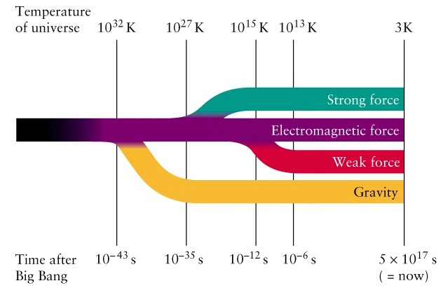
The role of the elementary interactions during the evolution¹ is depicted in Fig. 4. One can see that the splitting of one force after the Big Bang into the four kinds of forces that we know today, after $1.38 \times 10^{10}$ years of the evolution, happened in a very tiny fraction of the first second. Strong forces should be limited only to the scales (nucleon size of $\sim$10$^{-15}$ m) in the microworld, while general relativity models long-range gravitational interactions on very large scales of up to the size ($\sim$10$^{27}$ m) of the observed Universe. It is interesting that timescales are from 10$^{-24}$ s in atomic nuclei to nearly 10$^{18}$ s of the experimentally confirmed age of the Universe. This means a range of 42 orders of magnitude is the same as for spacescales; the masses span the range of about 83 orders of magnitude, between 10$^{-30}$ kg for the electron mass and about 10$^{53}$ kg for the of mass of the whole world ($\sim$10$^{80}$ baryons, mainly nucleons: protons and neutrons with mass of $\sim$10$^{-27}$ kg); this range is roughly twice as large as the time or space scale range.

Fig. 4

The grand unification theory (GUT) for the universe

Because the Universe has already expanded to that extremely huge size, gravitational forces (basically about 40 orders of magnitude weaker than strong nuclear forces) dominate the evolution of the Universe at present. However, at early stages of its evolution both forces resulted from an unknown simple law and could have been of a similar strength. The other long-range electromagnetic interactions between charged particles have already been unified with the short-range weak interactions responsible for the decay of nuclei (electroweak forces). Of course, the Grand Unification Theory (GUT) in Fig. 4 describing the unknown primordial force responsible for the creation of the Universe at a Planck scale of 10$^{-43}$ s will facilitate a better understanding of the physical processes at very early stages of the history of our world.

2.5 Quantum Models for the Creation of the Universe

Using the three available universal physical constants—namely the gravitational constant G, the speed of light c, and the Planck constant h, we can construct a quantity called a Planck length $l_{\mathrm P} = \sqrt{G \hslash / c^3}$, where $\hslash = h / (2 \pi )$. Another quantity $l_{\mathrm P}/c$ is the respective Planck time scale, $t_{\mathrm P}$. Because we do not have a quantum theory of gravitation quantum gravity a number of models for the creation creation of the Universe with the following characteristics have been proposed, including:

• The quantum model [2]

  creation from ‘nothing’, ex nihilo

• Noncommutative geometry [4]

  beginning is everywhere

• String theory, M-theory [30]

  collision of branes

• Cyclic (ekpyrotic) model [26, 27]

  big bangs and crunches

• Eternal chaotic inflation [5]

  bubble of universes.

The concept of the quantum wave function of the primordial Universe was put forward in [2]. This point of view was illustrated in a simple minisuperspace model with an invariant scalar field as the only gravitational degree of freedom. The authors of this model focus on the ground state with minimum excitation of an initial Universe on extremely small scales. Providing that the time is changed to imaginary values $\mathrm {i} t$, spacetime with a four-dimensional geometry becomes positive-defined. This allows us to obtain the path integral of the respective Euclidean action. In this way, the authors obtained finite nonzero probabilities of propagating from the ground (vacuum) state to the spectrum of possible excited states.

It is worth noting that below the Planck threshold $l_{\mathrm P} = 1.6 \times 10^{-35}$ m $\sim 10^{-35}$ m and $t_{\mathrm P} = 5.4 \times 10^{-44}$ s $\sim 10^{-43}$ s, in space and time, respectively, any time could be formally eliminated in the quantum model. In this scenario the Universe interpreted without any boundary conditions [2]. Moreover, because one can obtain the excited state from the vacuum state, they argue for the creation out of nothing, even ex nihilo. However, one should bear in mind that a quantum vacuum state is not actually ‘nothingness’—indeed it could be interpreted as a ‘sea’ of various possibilities [3].

An alternative interesting solution for the origin of spacetime on extremely small scales has been proposed in [4], where it was suggested that these critical values would correspond to a phase transition from a smooth commutative geometry to a rather singular noncommutative régime, with no space points and no time instances. Hence, noncommutative algebra is the other quantum gravity counterpart of the observable in the standard quantum theory, which can help in the application of quantization methods to the origin of the primordial Universe. Therefore, as one can paradoxically put it: the beginning is everywhere.

Following the M theory [30], in the context of an initial universe resulting from a collision of branes, another interesting non-standard cosmological scenario has been proposed in [26, 27]. According to their proposed model, the Universe undergoes a sequence of cosmic epochs each of which begins with a created world with a standard big bang event, followed by a slowly accelerating expansion with radiation and matter domination periods, but ends by contraction with a crunch. This model is called ekpyrotic, because in ancient Greece’s Stoic philosophy ecpirosi means ‘escape from fire’. This endless cycle of big bangs and crunches would avoid any particular singularity, but is able to explain the approximate homogeneity of distribution of mass, instead of a hypothetical inflation following the Planck epoch. It is worth noting that the model produces the recently observed flatness of spacetime geometry, providing the energy needed to restore the Universe from the same vacuum state in the next cycle. These authors also assure us that, owing to acceleration, this continuously repeating cyclic solution is an attractor [27].

Taking the wave function of the Universe [2], it can be shown that the large scale fluctuations of the quantum scalar field can generate an infinite process of self-reproducing primordial mini-universes. Therefore, one can suggest an eternally existing chaotic inflationary scenario, describing the Universe as a self-generating fractal that springs up from the multiverse [5]. Because it seems improbable that only one such Universe is chosen in reality by compactification during the expansion, it is argued that there exists a bubble of all possible universes that is always growing until a new universe is created by chaotic inflation in the bubble [5]. Therefore, there should exist an exponentially large number of causally disconnected mini-universes corresponding to all possible vacuum states followed by inflations. Admittedly, in the last two models time is eternal, but it is difficult to verify these models according to the criterion of falsifiability required for any scientific theory of Popper [24].

3 Nonlinear Dynamics and Fractals

In the second part of this paper we focus on nonlinear chaotic dynamics and fractals in a search for implications of an unknown nonlinear law related to a hidden order responsible for the creation of the Cosmos at the Planck epoch, see [12, ch. 3].

3.1 Deterministic Chaos

CHAOS ($\chi \acute{\alpha } \mathrm {o} \varsigma$) according to [29] is (see the excellent popular book by Stewart [28]):

• non-periodic long-term behavior

• in a deterministic system

• that exhibits sensitivity to initial conditions.

More precisely, we say that a bounded solution $\mathbf {x}(t)$ of a given dynamical system, $\dot{\mathbf {x}}=\mathbf {F}(\mathbf {x})$, is sensitive to initial conditions if there is a finite fixed distance $d > 0$ such that for any neighborhood $\Vert {\varDelta } \mathbf {x}(0)\Vert <\delta$, where $\delta >0$, there exists (at least some) other solutions $\mathbf {x}(t)$ + ${\varDelta }\mathbf {x}(t)$ for which for some time $t \ge 0$ we have $\Vert {\varDelta } \mathbf {x}(t)\Vert \ge d$. This means that there is a fixed distance d such that, no matter how precisely one specifies an initial state, there exists a solution of a dynamical system starting from a nearby state (at least one) that gets a distance d away.

Given $\mathbf {x}(\mathbf{t}) = \{x_1(t), \ldots , x_N(t)\}$, any positive finite value of Lyapunov exponents (or equivalently metric entropy)

$$\begin{aligned} \lambda _{k} = \lim _{t\rightarrow \infty } \frac{1}{t} \ln \Big |\frac{{\varDelta } {x}_{k}(t)}{{\varDelta } {x}_{k}(0)}\Big |, \end{aligned}$$

(1)

where $k=1, \ldots N$, implies chaos.

One example comes from the dynamics of irregular flow in viscous fluids, which is still not sufficiently well understood. It appears that the behavior of such systems can be rather complex: from equilibrium or regular (periodic) motion, through intermittency (where irregular and regular motions are intertwined) to nonperiodic behavior. Two types of such nonperiodic flows are possible, namely chaotic and hyperchaotic motions. As discovered by Lorenz (1963) deterministic chaos exhibits sensitivity to initial conditions leading to the unpredictability of the long-term behavior of the system (the ‘butterfly effect’) [6].

3.2 Hyperchaos

Hyperchaos is a more complex nonperiodic flow, which was discovered by Macek and Strumik (2010) [15] in the generalized Lorenz system previously proposed in [14]. Mathematical and physical aspects of this new low-dimensional model of hydromagnetic convection together with the detailed derivation from the basic partial differential equations, including the magnetic diffusion equations and naturally the anisotropic tension of the magnetic field lines, has been addressed in detail in [11].

Within the theory of dynamical systems transitions from fixed points to periodic or nonperiodic flows often occur in a given system through bifurcations, intermittency, resulting in a turbulent irregular behavior of the nonlinear system. In fact, we have identified type I and III intermittency [23] in the generalized Lorenz model of hydromagnetic convection, as also discussed in the papers [10, 14, 15]. It would be interesting to look for the remaining basic type II intermittency and the respective Hopf bifurcation in this model.

The following ordinary differential equations are obtained in the generalized Lorenz system [14]:

$$\begin{aligned} \left. \begin{array}{l} \dot{X} = -\sigma X + \sigma Y - \omega _0 W\\ \dot{Y} = -X Z + r X - Y\\ \dot{Z} = X Y - b Z\\ \dot{W} = \omega _0 X - \sigma _{\mathrm m}W. \end{array}\right\} \end{aligned}$$

(2)

In this simplified system, X(t) denotes a time amplitude of the potential of the velocity of a viscous horizontal fluid layer in the vertical gravitational field heated from below, with the normalized (dimensionless) Rayleigh number r, proportional to an initial temperature gradient $\delta T_0$, which is a control parameter of the system. Similarly, Y(t) and Z(t) correspond to the two lowest-order amplitudes of the deviation from the linear temperature profile of the layer (of height h) during the convection. The other parameter $\sigma = \nu / \kappa$ is the ratio of the kinematic viscosity $\nu$ to thermal conductivity $\kappa$ (the Prandtl number) characterizing the fluid and $b = 4/(1 + a^2$) is a geometric factor related to the aspect ratio a of the convected cells.

Admittedly, Lorenz (1963) only took three of several coefficients appearing in the lowest-order of the bispectral Fourier expansion, cf. [25]. In addition to the standard Lorenz system [6], a new time dependent variable W in (2) describes the profile of the magnetic field induced in the convected magnetized fluid. We have also introduced the second control parameter proportional to an initial horizontal magnetic field strength $B_0$ applied to the system, more precisely defined here as a basic dimensionless magnetic frequency $\omega _0 = {\upsilon _{\mathrm A0}}/\upsilon _0$, which is the ratio of the Alfvén velocity ${\upsilon _{\mathrm A0}} = {{B_0}} / {(\mu _0 \rho )^{1/2}}$, with a constant magnetic permeability $\mu _0$ and mass density $\rho$, to a characteristic speed $\upsilon _0 = 4 \pi \kappa / (a b h)$. Naturally, besides $\sigma = \nu / \kappa$, the magnetized viscous fluid is characterized by an analogue parameter $\sigma _{\mathrm m} = \eta / \kappa$, defined as the ratio of the magnetic resistivity $\eta$ to the thermal conductivity $\kappa$ (related to the magnetic Prandtl number, $Pr_\mathrm {m} = \sigma /\sigma _{\mathrm m}$).

Fig. 5

Color-coded dependence of the long-term asymptotic solutions of the generalized Lorenz system on the control parameters $\omega _0$ and r parameters (for $\sigma _{\mathrm m} = 3$). Equilibria (fixed points) (with a negative largest Lyapunov exponent, $\lambda _1<0$) are shown in black, periodic solutions ($\lambda _1=0$)—in violet/blue, and (nonperiodic) chaotic solutions ($\lambda _1>0$)—in a color, on the color bar scale, from violet to yellow. Fine structures are shown in the inset, as taken from Macek and Strumik (2014)

The results of our another paper illustrate how all these complex motions can be studied by analyzing this simple model [15, Fig. 1]. For example, for a chosen value of $\sigma _{\mathrm m} = 3$ (other parameters have the same values as for the classical Lorenz model, $\sigma = 10$, $b = 8/3$), Fig. 5 plots the largest Lyapunov exponent, calculated according to (1), depending on the control parameters $\omega _0$ and r. Convergence of the asymptotic solutions of (2) to equilibria described by fixed points ($\lambda _1<0$) is shown in black, to periodic (limit cycles) solutions ($\lambda _1=0$) – in violet/blue color (see the color bar for $\lambda _1=0$), to chaotic (nonperiodic) solutions ($\lambda _1>0$)—in a color, consistently with the color bar scale, from violet/blue to yellow. For the panel an enlargement of the region bounded by black lines is shown in the right-bottom part of plots. Fine structures are shown in the inset. This proves that various kinds of complex behavior are closely neighbored in the space of control parameters $\omega _0$ and r.

Convection appears naturally in plasmas, where electrically charged particles interact with the magnetic field. Therefore, the obtained results could be important for explaining dynamical processes in solar sunspots, planetary and stellar fluid interiors, and possibly for plasmas in nuclear fusion devices. Generally speaking, nonlinear differential equations or iterated discrete maps are useful models of some phenomena appearing naturally in the contexts in biology (e.g., animal population), economics, including finance theory, e.g., [22], and social sciences.

4 Fractals and Multifractals

Let us now move on to a basic concept of a fractal coined from the Latin adjective fractus and the corresponding verb frangere, which means ‘to break into irregular fragments’, see p. 4 of [20]; Mandelbrot (1982) always argued that fractal geometry is important for understanding the structure of nature describing, for example clouds, mountains, and coastlines, e.g. p. 1 of [20]. We can say that a fractal is a rough or fragmented geometrical object that can be subdivided in parts, each of which is (at least approximately) a reduced-size copy of the whole. Fractals are generally self-similar and independent of scale, described by a fractal dimension.

Fig. 6

Self-similar fractals of the Cantor (a) and Koch (b) sets

Namely, fractal structure is obtained recursively using a simple rule. The initial stages of the construction of two typical fractals in one-dimensional and two-dimensional space are schematically illustrated in Fig. 6 for a middle Cantor (a) and a Koch triangle (b) sets, respectively, which are also discussed in many textbooks, e.g. [21, 29]. First, as proposed by the German mathematician Georg Cantor in 1883, let us take a unit closed interval on a one-dimensional line and remove its open middle third, but necessarily leaving the endpoints behind. Second, we remove the open middle thirds of both closed smaller intervals, and in each of the following k-th step this produces $2^k$ closed (more and more narrower) intervals of length $(2/3)^k$, where $k = 1, \ldots , n$. Now imagine that the repetitions never end, one obtains the limiting set that consists of the intersection of all such closed intervals. Provided that $n \rightarrow \infty$, the resulting set has structure at arbitrarily small scales; the remaining elements during the construction are separated by various gaps. Surprisingly enough, two paradoxically opposite topological properties of the Cantor set (called also a dust) can be reconciled: the set itself is totally disconnected (without any closed intervals), but arbitrarily close to each elements one can always find another neighboring element (there are no isolated points).

Further, it is worth noting that each element of this set is specified by its location at successive steps, in the left (denoted by zero) or right (marked by one) fragment. One now sees that elements of the Cantor set are equivalent to various infinite sequences of zeros and ones, and can be put into one-to-one correspondence with the elements of the entire initial interval (in binary representation). Because common sense has some difficulty in comparing countable with uncountable infinity, this is somewhat strange that the Cantor set is uncountable, notwithstanding its total length equal to zero (the length of all the removed parts is equal one). Mainly because of this paradox, such sets are commonly called strange fractals, even though one can also construct fractals with length or in general volume (strictly a Lebesgue measure) different than zero. Similar fractal sets with zero Lebesgue measures constructed starting from a triangle or a full square on a two-dimensional plane were proposed by the Polish mathematician Wacław Sierpiński (1882–1969) in 1916.

Figure 6b shows another interesting snowflake curve obtained on a plane by adding onto sides of an initial equilateral triangle additional triangles that are three times smaller, after removing as before open middle thirds of any side. Blowing up this van Koch curve by a factor of three results in its length four times as large, and hence the length of perimeter of the triadic Koch island increases and becomes ultimately infinite, despite the fact that the area of course remains finite. Surprisingly, the arc length between any two elements of such a Koch set is also infinite. Therefore, because every element of this set is located infinitely far from any other element, the length cannot be used to identify the elements of such a strange fractal.

Mandelbrot (1982) noted that a fractal (Hausdorff) dimension,² which plays a central roles in case of fractal sets, exceeds the topological dimension, $D_{\mathrm T}$ [20]. Anyway, the concept of dimension should be modified as compared with a standard topological dimension useful in the Euclidean linear geometry. However, a somewhat different definition of a fractal set is generally accepted. The capacity dimension $D_{\mathrm F}$, which takes into account how many elements (cubes) of size l in phase space is needed to cover the set, is defined by

$$\begin{aligned} D_{\mathrm F} = \lim _{l \rightarrow 0} \frac{\ln N(l)}{\ln 1/l}. \end{aligned}$$

(3)

This means that fractal dimension is calculated by taking the limit of the quotient of the logarithm change in object size and the logarithm in scale as the limiting scale approaches zero. For example, the fractal dimensions of the Cantor and the Koch sets are $D_{\mathrm F} = \ln 2 / \ln 3 \approx 0.63$ (this means $D_{\mathrm F} > 0$) and $D_{\mathrm F} = \ln 4 / \ln 3 \approx 1.26$ ($> 1$) i.e., greater than the respective topological dimensions, $D_{\mathrm T} = 0$ and 1. As is known, the later non-integer dimension describes sufficiently well the length of the rocky western coast of Great Britain as a function of diminishing scale size, see [19]; in reality the lowest scale is admittedly limited.

4.1 Multifractal Models for Turbulence

A deviation from a strict self-similarity is also called intermittency, and that is why a generalized two-scale weighted Cantor set has been applied for modeling intermittent turbulence in fluids [8, 9].

In fact, this complex process can be described by the generalized weighted Cantor set, as illustrated in Fig. 7 taken from [8]. In the first step of the two-scale model construction, we have two eddies of sizes $l_{1}$ and $l_{2}$ satisfying $p_{1}/l_{1} + p_{2}/l_{2} = 1$. Therefore, the initial energy flux $\varepsilon _0$ is transferred to these eddies with the different proportions: $\varepsilon _0 p_{1}/l_{1}$ and $\varepsilon _0 p_{2}/l_{2}$. In the next step the kinetic or magnetic energy flux is divided between four eddies in the following way: $\varepsilon _0 (p_{1}/l_{1})^{2}$, $\varepsilon _0 p_{1}p_{2}/(l_{1}~l_{2})$, $\varepsilon _0 p_{2} p_{1}/(l_2 l_1)$, and $\varepsilon _0 (p_{2}/l_2)^{2}$. At nth step we have $N = 2^n$ eddies and partition of energy $\varepsilon$ can be described by the binomial formula, e.g., [9]:

$$\begin{aligned} \varepsilon = \sum \limits _{i=1}^{N}\varepsilon _{i} = \varepsilon _0 \sum \limits _{k=0}^{n}{n\atopwithdelims ()k} \left( \frac{p_{1}}{l_{1}} \right) ^{(n-k)} \left( \frac{p_{2}}{l_{2}}\right) ^{k}. \end{aligned}$$

(4)

Fig. 7

The generalized two-scale weighted Cantor set model for turbulence

For any real number $-\infty< q < +\infty$, one obtains the generalized dimension defined by $D_q = \tau (q)/(q-1)$ by solving numerically the transcendental equation, e.g., [21],

$$\begin{aligned} \frac{p_1^{q}}{l_{1}^{\tau (q)}}+\frac{p_2^{q}}{l_{2}^{\tau (q)}} = 1, \end{aligned}$$

(5)

which is only somewhat more general than the analytical solution. In particular, for the one-scale multifractal model with $l_1 = l_2 = \lambda$, we have $D _q = - \ln (p_{1}^q + p_{2}^q) / \ln \lambda$, and a special case for $\lambda$ = 1/2 is called P-model, as classified on the right side of Fig. 7. We see that only for equal scales together with equal weights ($p_1 = p_2$ = 1/2) there is no multifractality, and we have a monofractal with a fractal dimension given by (3).

5 Implications for Cosmology and the Creation of the Universe

This method was extensively used in various situations in solar wind magnetized plasmas based on space missions penetrating various regions of the solar system, see [9, 13, 16, 17]. In this way, based on a wealth of data acquired from Helios in the inner heliosphere and especially from deep space Voyager 1 and 2 spacecraft in the outer heliosphere, we have shown that turbulence is intermittent in the entire heliospheric system, even at the heliospheric boundaries [18]. However, it appears that the heliosphere is immersed in a relatively quiet very local interstellar medium. Therefore, after crossing the heliopause (on 25 August 2012), which is the ultimate boundary separating the heliospheric and interstellar plasmas, Voyager 1 only detected smoothly varying magnetic fields. As expected this change in the behavior of plasma parameters (with a frozen-in magnetic field) was confirmed by the crossing of the heliopause by Voyager 2 in 2018.

Moreover, based on scientific experience, I have argued that a simple but possibly nonlinear law [7], within the theory of chaos and (multi-)fractals, can describe a hidden order for the creation of the Cosmos, at the Planck epoch, when space (at a scale of 10$^{-35}$ m) and time (10$^{-43}$ s) originated, see [12, p. 3.4].

6 Conclusions

To summarize, based on space, astrophysical, and even cosmological applications, one can say that

• Nonlinear systems exhibit complex phenomena, including bifurcation, intermittency, and chaos.

• Fractals can describe complex shapes in the real word.

• Strange chaotic attractors have fractal structure and are sensitive to initial conditions.

• Within the complex dynamics of the fluctuating intermittent parameters of turbulent media there is a detectable, hidden order described by a generalized Cantor set that exhibits a multifractal structure.

References

P.B. Abbot et al., Observation of gravitational waves from a binary black hole merger. Phys. Rev. Lett. 116, 061102 (2016). https://doi.org/10.1103/PhysRevLett.116.061102
J.B. Hartle, S.W. Hawking, Wave function of the Universe. Phys. Rev. D 28, 2960–2975 (1983). https://doi.org/10.1103/PhysRevD.28.2960
M. Heller, Ultimate Explanations of the Universe (Springer, Berlin, Heidelberg, 2009). https://doi.org/10.1007/978-3-642-02103-9
M. Heller, W. Sasin, Noncommutative structure of singularities in general relativity. J. Math. Phys. 37, 5665–5671 (1996). https://doi.org/10.1063/1.531733
A.D. Linde, Eternally existing self-reproducing chaotic inflationary universe. Phys. Lett. B 175, 395–400 (1986). https://doi.org/10.1016/0370-2693(86)90611-8
E.N. Lorenz, Deterministic nonperiodic flow. J. Atmos. Sci. 20, 130–141 (1963). https://journals.ametsoc.org/view/journals/atsc/20/2/1520-0469_1963_020_0130_dnf_2_0_co_2.xml
W.M. Macek, On being and non-being in science, philosophy, and theology, in Interpretazioni del reale. Teologia, filosofia e scienze in dialogo (Interpretations of Reality: a Dialogue among Theology, Philosophy, and Sciences). Pontificia Università Lateranense (Pontifical Lateran University), Rome, Italy, ed. by P. Coda, R. Presilla. Quaderni Sefir, vol. 1 (2000), pp. 119–132
W.M. Macek, Multifractality and intermittency in the solar wind. Nonlinear Process. Geophys. 14(6), 695–700 (2007). https://doi.org/10.5194/npg-14-695-2007
W.M. Macek, Multifractal turbulence in the heliosphere, in Exploring the Solar Wind. ed. by M. Lazar (Intech, Croatia, 2012), pp. 143–168
W.M. Macek, Intermittency in the generalized Lorenz model, in Chaotic Modeling and Simulation, ed. by C. Skiadas. Int. J. Nonlinear Sci. 4, 323–328 (2015). http://www.cmsim.eu/
W.M. Macek, Nonlinear dynamics and complexity in the generalized Lorenz system. Nonlinear Dyn. 94(4), 2957–2968 (2018). https://doi.org/10.1007/s11071-018-4536-z
W.M. Macek, The Origin of the World: Cosmos or Chaos? (Cardinal Stefan Wyszyński University (UKSW) Scientific Editions, 2020). ISBN 978-83-8090-686-0, e-ISBN 978-83-8090-687-7
W.M. Macek, A. Wawrzaszek, Evolution of asymmetric multifractal scaling of solar wind turbulence in the outer heliosphere. J. Geophys. Res. 114(A3), A03108 (2009). https://doi.org/10.1029/2008JA013795
W.M. Macek, M. Strumik, Model for hydromagnetic convection in a magnetized fluid. Phys. Rev. E 82(2), 027301 (2010). https://doi.org/10.1103/PhysRevE.82.027301
W.M. Macek, M. Strumik, Hyperchaotic intermittent convection in a magnetized viscous fluid. Phys. Rev. Lett. 112(7), 074502 (2014). https://doi.org/10.1103/PhysRevLett.112.074502
W.M. Macek, A. Wawrzaszek, V. Carbone, Observation of the multifractal spectrum at the termination shock by Voyager 1. Geophys. Res. Lett. 38, L19103 (2011). https://doi.org/10.1029/2011GL049261
W.M. Macek, A. Wawrzaszek, V. Carbone, Observation of the multifractal spectrum in the heliosphere and the heliosheath by Voyager 1 and 2. J. Geophys. Res. 117, A12101 (2012). https://doi.org/10.1029/2012JA018129
W.M. Macek, A. Wawrzaszek, L.F. Burlaga, Multifractal structures detected by Voyager 1 at the heliospheric boundaries. Astrophys. J. Lett. 793, L30 (2014). https://doi.org/10.1088/2041-8205/793/2/L30
B.B. Mandelbrot, How long is the coast of Britain? Statistical self-similarity and fractional dimension. Science 156(3775), 636–638 (1967). https://doi.org/10.1126/science.156.3775.636
B.B. Mandelbrot, The Fractal Geometry of Nature (W. H. Freeman, New York, 1982)
E. Ott, Chaos in Dynamical Systems (Cambridge Univ. Press, Cambridge, 1993)
E.E. Peters, Chaos and Order in the Capital Markets: A New View of Cycles, Prices, and Market Volatility, 2nd edn. (Addison-Wesley, Reading, MA, 1996). Wiley, 978-0-471-13938-6
Y. Pomeau, P. Manneville, Intermittent transition to turbulence in dissipative dynamical systems. Commun. Math. Phys. 74, 189–197 (1980). https://doi.org/10.1007/BF01197757
K.R. Popper, The Logic of Scientific Discovery (Routledge, London, New York, 1959)
B. Saltzman, Finite amplitude free convection as an initial value problem—I. J. Atmos. Sci. 19, 329–341 (1962). https://journals.ametsoc.org/view/journals/atsc/19/4/1520-0469_1962_019_0329_fafcaa_2_0_co_2.xml
P.J. Steinhardt, N. Turok, A cyclic model of the universe. Science 296, 1436–1439 (2002). https://doi.org/10.1126/science.1070462
P.J. Steinhardt, N. Turok, Cosmic evolution in a cyclic universe. Phys. Rev. D 65(12), 126003 (2002). https://doi.org/10.1103/PhysRevD.65.126003
I. Stewart, Does God Play Dice?: The New Mathematics of Chaos (Blackwell Publishers, 1990)
S.H. Strogatz, Nonlinear Dynamics and Chaos: With Applications to Physics, Biology, Chemistry, and Engineering (Addison-Wesley, Reading, MA, 1994)
E. Witten, String theory dynamics in various dimensions. Nucl. Phys. B 443, 85–126 (1995). https://doi.org/10.1016/0550-3213(95)00158-O
Acknowledgements
The research studies on chaos and turbulence in space plasmas have been funded in part by the National Science Centre (NCN), Poland, through grants 2014/15/B/ST9/04782 and 2021/41/B/ST10/00823. I would like to thank the NASA/WMAP Science and ESA/NASA Planck Teams for providing the schematic of the Evolution of the Universe and the illustrations of gravitation and geometry.
Author information
Authors and Affiliations
Corresponding author
Editor information
Editors and Affiliations
Rights and permissions
Open Access This chapter is licensed under the terms of the Creative Commons Attribution 4.0 International License (http://creativecommons.org/licenses/by/4.0/), which permits use, sharing, adaptation, distribution and reproduction in any medium or format, as long as you give appropriate credit to the original author(s) and the source, provide a link to the Creative Commons license and indicate if changes were made.
The images or other third party material in this chapter are included in the chapter's Creative Commons license, unless indicated otherwise in a credit line to the material. If material is not included in the chapter's Creative Commons license and your intended use is not permitted by statutory regulation or exceeds the permitted use, you will need to obtain permission directly from the copyright holder.
Copyright information
© 2022 The Author(s)
About this paper
Cite this paper
Macek, W.M. (2022). On the Origin of the Universe: Chaos or Cosmos?. In: Skiadas, C.H., Dimotikalis, Y. (eds) 14th Chaotic Modeling and Simulation International Conference. CHAOS 2021. Springer Proceedings in Complexity. Springer, Cham. https://doi.org/10.1007/978-3-030-96964-6_21
Download citation
DOI: https://doi.org/10.1007/978-3-030-96964-6_21
Published:
Publisher Name: Springer, Cham
Print ISBN: 978-3-030-96963-9
Online ISBN: 978-3-030-96964-6
eBook Packages: Physics and AstronomyPhysics and Astronomy (R0)