
Abstract
Induction and coinduction are both used extensively within mathematics and computer science. Algebraic formulations of these principles make the duality between them apparent, but do not account well for the way they are commonly used in deduction. Generally, the formalization of these reasoning methods employs inference rules that express a general explicit (co)induction scheme. Non-well-founded proof theory provides an alternative, more robust approach for formalizing implicit (co)inductive reasoning. This approach has been extremely successful in recent years in supporting implicit inductive reasoning, but is not as well-developed in the context of coinductive reasoning. This paper reviews the general method of non-well-founded proofs, and puts forward a concrete natural framework for (co)inductive reasoning, based on (co)closure operators, that offers a concise framework in which inductive and coinductive reasoning are captured as we intuitively understand and use them. Through this framework we demonstrate the enormous potential of non-well-founded deduction, both in the foundational theoretical exploration of (co)inductive reasoning and in the provision of proof support for (co)inductive reasoning within (semi-)automated proof tools.
You have full access to this open access chapter, Download conference paper PDF
1 Introduction
The principle of induction is a key technique in mathematical reasoning that is widely used in computer science for reasoning about recursive data types (such as numbers or lists) and computations. Its dual principle—the principle of coinduction [49, 69, 70]—is not as widespread, and has only been investigated for a few decades, but still has many applications in computer science, e.g. [39, 42, 52, 55,56,57, 82]. It is mainly used for reasoning about coinductive data types (codata), which are data structures containing non-well-founded elements, e.g., infinite streams or trees. One prominent application of coinduction is as a generic formalism for reasoning about state-based dynamical systems, which typically contain some sort of circularity. It is key in proofs of the bisimulation of state-transition systems (i.e., proving that two systems are behaviorally equivalent) and is a primary method for reasoning about concurrent systems [53].
A duality between induction and coinduction is observed when formulating them within an algebraic, or categorical, framework, e.g., [64, 69,70,71]. Whereas induction corresponds to a least-fixed-point semantics (or initial algebras), coinduction corresponds to a greatest-fixed-point semantics (or final coalgebras). However, such an algebraic formulation does not account well for the way these principles are commonly used in deduction, where they are usually applied in different ways: induction to prove properties of certain collections, and coinduction to show equivalences between processes and systems.
Since the principle of induction is so well-known, induction methods are relatively well-developed. They are available in most (semi-)automated deduction systems, and tools for the formal verification of software and hardware such as theorem provers. Generally, implementations of the induction method employ one or more inference rules that express a general explicit induction scheme that holds for the elements being reasoned over. That is, to prove that some property, say P, holds for all elements in an inductively defined set, we (i) show that it holds for the initial elements, and (ii) show that P is preserved in the inductive generation of new elements. A side-effect of such implementations is that in applying inductive reasoning, the induction invariant must be provided explicitly. While advanced provers offer powerful facilities for producing and manipulating inductive goals, this still poses a major automation challenge. This formalization of the induction principle uses the classical notion of formal proofs invoked in standard theorem provers. There, proofs are well-founded trees, starting at the goal and reaching axioms while proceeding by applications of inference rules.
A more robust and natural alternative formalization of inductive reasoning is implicit induction, which avoids the need for explicitly specifying induction invariants. This form of reasoning is enabled by extending the standard notion of well-founded, finite proof trees into non-well-founded proof trees, where the presence of cycles can be exploited instead of cluttering the proof with explicit inductive invariants. For example, to prove P(x) using implicit induction, one repeatedly decomposes the goal into subgoals that are either provable in the standard way (via well-founded subtrees) or reducible back to P(x). This alternative has deep historic roots (originating in Fermat’s infinite-descent method) and recently has seen a flourishing of its proof theory via cyclic proof systems.
Non-well-founded proof theory and its cyclic fragment (comprising only of finite and regular proofs) have been extremely successful in recent years in supporting implicit inductive reasoning. For one, the non-well-founded approach has been used to obtain (optimal) cut-free completeness results for highly expressive logics, such as the \(\mu \)-calculus [3, 34, 35, 37] and Kleene algebra [32, 33], providing further evidence of its utility for automation. Other works focus on the structural proof theory of non-well-founded systems, where these promote additional insights into standard proof-theoretical questions by separating local steps of deductive inference from global well-foundedness arguments. In particular, syntactic cut elimination for non-well-founded systems has been studied extensively in the linear logic settings [7, 41]. Much work has been devoted to the formal study of explicit versus implicit forms of induction in various logical settings including the \(\mu \)-calculus [7, 62, 72, 75], systems for arithmetics [31, 74], and first-order logics with inductive definitions [14, 19, 19]. The latter offers a system parameterized by a set of inductive predicates with associated rules, rather than a single rule for induction as with the others. The cyclic machinery has also been used to effectively search for proofs of inductive properties and automatically verify properties of inductive programs, especially in the context of separation logic [16,17,18, 68, 78].
Unlike induction, the coinduction principle has not been so fully and naturally incorporated into major theorem provers, but it has gained importance and attention in recent years. As noted by Basold, Komendantskaya, and Li: “it may be surprising that automated proof search for coinductive predicates in first-order logic does not have a coherent and comprehensive theory, even after three decades...” [8]. Automated provers, to the best of our knowledge, currently do not offer any support for coinduction, and while coinductive data types have been implemented in interactive theorem provers (a.k.a. proof assistants) such as Coq [11, 47, 83], Nuprl [30], Isabelle [12, 13, 38, 81], Agda [1], Lean [4], and Dafny [54], the treatment of these forms of data is often partial. These formalizations, as well as other formal frameworks that support the combination of induction and coinduction, e.g., [6, 46, 61, 80], generally rely on making (co)invariants explicit within proofs. But just as inductive reasoning is naturally captured via proof cycles, cyclic systems seem to be particularly well-suited for also encompassing the implicit notion of coinduction. Nonetheless, while non-well-founded proof theory has been very successful in supporting inductive reasoning, this proof method has not been equally incorporated and explored in the context of coinductive reasoning. Some notable cyclic systems that do support coinduction in various settings include [2, 36, 58, 67, 72]. Another related framework is that of Coq’s parameterized coinduction [47, 83], which offers a different, but highly related, implicit nature of proofs (based on patterns within parameters, rather than within proof sequents).
This paper reviews the general method of non-well-founded proof theory, focusing on its use in capturing both implicit inductive and coinductive reasoning. Throughout the paper we focus on one very natural and simple logical framework to demonstrate the benefits of the approach—that of the transitive (co)closure logic. This logic offers a succinct and intuitive dual treatment to induction and coinduction, while still supporting their common practices in deduction, making it great for prototyping. More specifically, it has the benefits of (1) conciseness: no need for a separate language or interpretation for definitions, nor for fully general least/greatest-fixed-point operators; (2) intuitiveness: the concept of transitive closure is basic, and the dual closure is equally simple to grasp, resulting in a simpler metatheory; (3) illumination: similarities, dualities, and differences between induction and coinduction are clearly demonstrated; and (4) naturality: local reasoning is rudimentary, and the global structure of proofs directly reflects higher-level reasoning. The framework presented is based on ongoing work by Reuben Rowe and the author, some of which can be found in [23, 26, 28, 29]. We conclude the paper by briefly discussing two major open research questions in the field of non-well-founded theory: namely, the need for a user-friendly implementation of the method into modern proof assistants, in order to make it applicable and to facilitate advancements in automated proof search and program verification, and the task of determining the precise relationship between systems for cyclic reasoning and standard systems for explicit reasoning.
2 The Principles of Induction and Coinduction
A duality between the induction principle and the coinduction principle is clearly observed when formulating them within an algebraic, or categorical, framework. This section reviews such a general algebraic formalization (Section 2.1), and then presents transitive (co)closure logic, which will serve as our running example throughout this paper as it provides simple, yet very intuitive, inductive and coinductive notions (Section 2.2).
2.1 Algebraic Formalization of Induction and Coinduction
Both the induction principle and the coinduction principle are usually defined algebraically via the concept of fixed points, where the definitions vary in different domains such as order theory, set theory or category theory. We opt here for a set-theoretical representation for the sake of simplicity, but more general representations, e.g., in a categorical setting, are also well-known [71].
Let \(\varPsi :\wp (D)\rightarrow \wp (D)\) be a monotone operator on sets for some fixed domain D (where \(\wp (D)\) denotes the power set of \(D\)). Since \((\wp (D), \subseteq )\) is a complete lattice, by the Knaster–Tarski theorem, both the least-fixed point and greatest-fixed point of \(\varPsi \) exist. The least-fixed point (\({{\,\mathrm{\mu }\,}}\)) is given by the intersection of all its prefixed points—that is, those sets A satisfying \(\varPsi (A) \subseteq A\)—and, dually, the greatest-fixed point (\({{\,\mathrm{\nu }\,}}\)) is given by the union of all its postfixed points—that is, those sets A satisfying \(A \subseteq \varPsi (A)\). These definitions naturally yield corresponding induction and coinduction principles.
-
Induction Principle: \(~ \qquad \qquad \varPsi (A) \subseteq A \implies {{\,\mathrm{\mu }\,}}(\varPsi ) \subseteq A\)
-
Coinduction Principle: \(\qquad \quad A \subseteq \varPsi (A) \implies A \subseteq {{\,\mathrm{\nu }\,}}(\varPsi )\)
The induction principle states that \({{\,\mathrm{\mu }\,}}(\varPsi )\) is contained in every \(\varPsi \)-closed set, where a set A is called \(\varPsi \)-closed if, for all \(a \in A\) and \(b \in D\), \((a, b) \in \varPsi (A)\) implies \(b \in A\) (which means that \( {{\,\mathrm{\mu }\,}}(\varPsi ) = \bigcap \{ A \,\mid \, \varPsi (A) \subseteq A \}\)). The coinduction principle dually states that \({{\,\mathrm{\nu }\,}}(\varPsi )\) contains every \(\varPsi \)-consistent set, where a set A is called \(\varPsi \)-consistent if, for all \(a \in A\), there is some \(b \in D\) such that both \((a, b) \in \varPsi (A)\) and \(b \in A\) (which means that \( {{\,\mathrm{\nu }\,}}(\varPsi ) = \bigcup \{ A \,\mid \, A \subseteq \varPsi (a) \}\)).
The intuition behind an inductively defined set is that of a “bottom-up” construction. That is, one starts with a set of initial elements and then applies the constructor operators finitely many times. One concrete example of an inductively defined set is that of finite lists, which can be constructed starting from the empty list and one constructor operator that adds an element to the head of the list. The finiteness restriction stems from the fact that induction is the smallest subset that can be constructed using the operators. Using the induction principle, one can show that all elements of an inductively defined set satisfy a certain property, by showing that the property is preserved for each constructor operator. A coinductively defined set is also constructed by starting with a set of initial elements and applying the constructor operators, possibly infinitely many times. One example, which arises from the same initial element and constructors as the inductive set of lists, is that of possibly infinite lists, i.e. the set that also contains infinite streams. The fact that we can apply the operators infinitely many times is due to coinduction being the largest subset that can (potentially) be constructed using the operators. Using the coinduction principle, one can show that an element is in a coinductively defined set.
2.2 Transitive (Co)closure Operators
Throughout the paper we will use two instances of fixed points that provide a minimal framework which captures applicable forms of inductive and coinductive reasoning in an intuitive manner, and is more amenable for automation than the full theory of fixed points. This section introduces these fixed points and discusses the logical framework obtained by adding them to first-order logic.
Definition 1 ((Post-)Composition Operator)
Given a binary relation, X, \(\varPsi _{X}\) is an operator on binary relations that post-composes its input with X, that is \(\varPsi _{X}(R) = X \cup (X \circ R) = \{ (a, c) \,\mid \, (a, c) \in X \vee \exists b \mathbin {.}(a, b) \in X \wedge (b, c) \in R \}\).
Because unions and compositions are monotone operators over a complete lattice, so are composition operators, and therefore both \({{\,\mathrm{\mu }\,}}(\varPsi _{X})\) and \({{\,\mathrm{\nu }\,}}(\varPsi _{X})\) exist. A pair of elements, (a, b), is in \({{\,\mathrm{\mu }\,}}(\varPsi _{X})\) when b is in every X-closed set that can be reached by some X-steps from a, which is equivalent to saying that there is a finite (non-empty) chain of X steps from a to b. A pair of elements, (a, b), is in \({{\,\mathrm{\nu }\,}}(\varPsi _{X})\) when there exists a set A that contains a such that the set \(A \setminus \{b\}\) is X-consistent, which is equivalent to saying that either there is a finite (non-empty) chain of X steps from a to b, or there is an infinite chain of X steps starting from a.
The \({{\,\mathrm{\mu }\,}}(\varPsi _{X})\) operator is in fact the standard transitive closure operator. Extending first-order logic (FOL) with the addition of this transitive closure operator results in the well-known transitive closure logic (a.k.a. ancestral logic), a generic, minimal logic for expressing finitaryFootnote 1 inductive structures [5, 23,24,25, 48, 73]. Transitive closure (\(\mathsf {TC}\)) logic was recently extended with a dual operator, called transitive co-closure, that corresponds to \({{\,\mathrm{\nu }\,}}(\varPsi _{X})\) [27]. The definition below presents the syntax and semantics of the extended logic, called Transitive (co)Closure logic, or \(\mathsf {TcC}\) logic.
Definition 2
( \(\mathsf {TcC}\)Logic). For \(\sigma \) a first-order signature, let s, t and P range over terms and predicate symbols over \(\sigma \) (respectively), and let \(M\) be a structure for \(\sigma \), and \(\nu \) a valuation in \(M\).
-
Syntax. The language \(\mathcal {L}_{TcC}\) (over \(\sigma \)) is given by the following grammar:

where the variables x, y in the formulas \(( TC _{{x},{y}}\,{\varphi })(s, t)\) and \((\mathop { TC ^{\mathsf {op}}_{{x},{y}}} {\varphi })(s, t)\) are distinct and are bound in the subformula \(\varphi \).
-
Semantics. The satisfaction relation \(M, \nu \models \varphi \) extends the standard satisfaction relation of classical first-order logic with the following clauses:
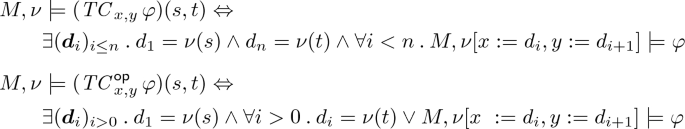
where \(\nu [x_1 := d_n, \ldots , x_n := d_n]\) denotes the valuation that maps \(x_i\) to \(d_i\) and behaves as \(\nu \) otherwise; \(\varphi \left\{ {\frac{t_{1}}{x_{1}}, \ldots , \frac{t_{n}}{x_{n}}} \right\} \) denotes simultaneous substitution; and \((\mathbf {d}_{i})_{i \le n}\) and \((\mathbf {d}_{i})_{i > 0}\) denote, respectively, non-empty finite and (countably) infinite sequences of elements from the domain.


Intuitively, the formula \(( TC _{{x},{y}}\,{\varphi })(s, t)\) asserts that there is a (possibly empty) finite \(\varphi \)-path from s to t, while the formula \((\mathop { TC ^{\mathsf {op}}_{{x},{y}}} {\varphi })(s, t)\) asserts that either there is a (possibly empty) finite \(\varphi \)-path from s to t, or an infinite \(\varphi \)-path starting at s. For simplicity of presentation we take here the reflexive forms of the closure operators, which yields the following correspondence.Footnote 2
Proposition 1
Let \([\![{\varphi }]\!]^{M,\nu }_{x,y} := \{ (a, b) \,\mid \, M, \nu [x := a, y := b] \models \varphi \}\).
-
(i)
\(M, \nu \models ( TC _{{x},{y}}\,{\varphi })(s, t) \quad \Leftrightarrow ~~ \nu (s)=\nu (t)\) or \((\nu (s), \nu (t)) \in {{\,\mathrm{\mu }\,}}(\varPsi _{[\![{\varphi }]\!]^{M,\nu }_{x,y}})\).
-
(ii)
\(M, \nu \models (\mathop { TC ^{\mathsf {op}}_{{x},{y}}} {\varphi })(s, t) ~~~\Leftrightarrow ~~ \nu (s) = \nu (t)\) or \((\nu (s), \nu (t)) \in {{\,\mathrm{\nu }\,}}(\varPsi _{[\![{\varphi }]\!]^{M,\nu }_{x,y}})\).
Note that, unlike the situation in standard fixed-point logics, the two closure operators are not inter-definable. The \( TC \) operator is definable in arithmetics (i.e. in Peano Arithmetics, PA), but the \( TC ^{\mathsf {op}}\) operator is not.
Thus, \(\mathsf {TcC}\) logic is subsumed by fixed-point logics, such as the first-order \(\mu \)-calculus [64], but the concept of the transitive (co)closure is intuitively simpler than that of general fixed-point operators, and it does not require any syntactic restrictions to ensure monotonicity. In fact, due to its complexity and generality, the investigation of the full first-order \(\mu \)-calculus tends to focus only on variants and fragments, and is mainly concentrated on the logical and model-theoretic aspects, lacking a comprehensive proof theory.Footnote 3 Another reason for focusing on these (co)closure operators is that they allow for the embedment of many forms of inductive and coinductive reasoning within one concise logical framework. Thus, while other extensions of FOL with inductive definitions are a priori parametrized by a set of inductive definitions [19, 59, 60, 79], bespoke induction principles do not need to be added to \(\mathsf {TcC}\) logic; instead, applicable (co)induction schemes are available within a single, unified language. This conciseness allows the logic to be formally captured using one fixed set of inference rules, and thus makes it particularly amenable for automation. Moreover, in \(\mathsf {TcC}\) logic, the same signature is shared for both inductive and coinductive data, making certain aspects of the relationship between the two principles more apparent.
Defining infinite structures via the coclosure operators in \(\mathsf {TcC}\) logic leads to a symmetric foundation for functional languages where inductive and coinductive data types can be naturally mixed. For example, using the standard list constructors (the constant \(\mathsf {nil}\) and the (infix) binary function symbol ‘\({{\,\mathrm{{:}{:}}\,}}\)’) and their axiomatization, the collections of finite lists, possibly infinite lists, and infinite lists (i.e., streams) are straightforwardly definable as follows.

\(\mathsf {TcC}\) logic also naturally captures properties of, and functions on, streams [29].
3 Non-well-founded Deduction for Induction
This section presents the general method of non-well-founded proof theory (Section 3.1), and then provides a concrete example of a non-well-founded proof system for inductive reasoning in the setting of the transitive closure (Section 3.2), where the implicit form of inductive reasoning is then compared against the explicit one. Note that this section first presents the proof theory only for \(\mathsf {TC}\) logic, which is the inductive fragment of \(\mathsf {TcC}\) logic, i.e., the one based only on the transitive closure operator.
3.1 Non-well-founded Proof Theory
The method of non-well-founded proofs provides an alternative approach to explicit inductive reasoning by exploiting the fact that there are no infinite descending chains of elements of well-ordered sets. Clearly, not all non-well-founded proof trees constitute a valid proof, i.e. a proof of the validity of the conclusion in the root. A proof tree that simply has one loop over the conclusion or one that repeatedly uses the substitution or permutation rules to obtain cycles are examples of non-well-founded proof trees that one would not like to consider as valid. Thus, a non-well-founded proof tree is allowed to be infinite, but to be considered as a valid proof, it has to obey an additional requirement that prevents such unsound deductions. Hence, non-well-founded proofs are subject to the restriction that every infinite path in the proof admits some infinite descent. Intuitively, the descent is witnessed by tracing syntactic elements, terms or formulas, for which we can give a correspondence with elements of a well-founded set. In this respect, non-well-founded proof theory enables a separation between local steps of deductive inference and global well-foundedness arguments, which are encoded in traces of terms or formulas through possibly infinite derivations.
Below we present proof systems in the style of sequent calculus. Sequents are expressions of the form \({\varGamma } \Rightarrow {\varDelta }\), for finite sets of formulas \(\varGamma \) and \(\varDelta \). We write \(\varGamma , \varphi \) as a shorthand for \(\varGamma \cup \{ \varphi \}\), and \(\mathsf {fv}(\varGamma )\) for the set of free variables of the formulas in \(\varGamma \). A sequent \({\varGamma } \Rightarrow {\varDelta }\) is valid if and only if the formula \(\bigwedge _{\varphi \in \varGamma } \varphi \rightarrow \bigvee _{\psi \in \varDelta } \psi \) is.
Let \(\mathcal {S}\) be a collection of inference rules. First, we define the notion of a non-well-founded proof tree, a pre-proof, based on \(\mathcal {S}\).
Definition 3 (Pre-proofs)
A pre-proof in \(\mathcal {S}\) is a possibly infinite derivation tree formed using the inference rules of \(\mathcal {S}\). A path in a pre-proof is a possibly infinite sequence of sequents, \(s_0, s_1, \ldots (, s_n)\), such that \(s_0\) is the root sequent of the proof, and \(s_{i+1}\) is a premise of \(s_i\) in the derivation tree for each \(i < n\).
As mentioned, not every pre-proof is a proof: only those in which there is some notion of infinite descent in every infinite branch, which allows one to formalize inductive arguments. To make this concrete, one picks some syntactic element, which can be formulas or terms, to be tracked through a pre-proof. We call such elements traced elements. The intuition behind picking the traced elements is that eventually, when we are given a pre-proof, we could trace these elements through the infinite branches, and map them into some well-founded set. This is what underpins the soundness of the non-well-founded method, as explained below. Given certain traced elements, we inductively define a notion of trace pairs which corresponds to the appearances of such traced elements within applications of the inference rules throughout the proof. That is, for traced elements, \(\tau , \tau '\), and a rule with conclusion s and a premise \(s'\) such that \(\tau \) appears in s and \(\tau '\) appears in \(s'\), \((\tau , \tau ')\) is said to be a trace pair for \((s, s')\) for certain rule applications, and there has to be at least one case identified as a progressing trace pair. The progression intuitively stands for the cases in which the elements of the trace pair are mapped to strictly decreasing elements of the well-founded set. We provide a concrete example of traced elements and a trace pair definition in the transitive closure setting in Section 3.2.
Definition 4 (Traces)
A trace is a (possibly infinite) sequence of traced elements. We say that a trace \(\tau _{1}, \tau _{2}, \ldots (, \tau _{n})\) follows a path \(s_{1}, s_{2}, \ldots (, s_{m})\) in a pre-proof \(\mathcal {P}\) if, for some \(k \ge 0\), each consecutive pair of formulas \((\tau _{i}, \tau _{i+1})\) is a trace pair for \((s_{i+k}, s_{i+k+1})\). If \((\tau _{i}, \tau _{i+1})\) is a progressing pair, then we say that the trace progresses at i, and we say that the trace is infinitely progressing if it progresses at infinitely many points.
Proofs, then, are pre-proofs which satisfy a global trace condition.
Definition 5 (Infinite Proofs)
A proof is a pre-proof in which every infinite path is followed by some infinitely progressing trace.
We denote by \(\mathcal {S}^\infty \) the non-well-founded proof system based on the rules in \(\mathcal {S}\).
The general soundness argument for such infinite systems follows from a combination of standard local soundness of the inference rules in \(\mathcal {S}\) together with a global soundness argument via an infinite descent-style construction, due to the presence of infinitely progressing traces for each infinite path in a proof. One assumes for contradiction that the conclusion of the proof is invalid, which, by the local soundness of the rules, entails the existence of an infinite sequence of counter-models, going along an infinite branch. Then, one demonstrates a mapping of these models into a well-founded set, \((D,<)\), which decreases while following the sequence of counter-models, and strictly decreases when going over progression points. But then, by the global trace condition, there exists an infinitely descending chain in D, which of course yields a contradiction.
While a full infinitary proof system is clearly not effective, effectiveness can be obtained by restricting consideration to the cyclic proofs, i.e., those that are finitely representable. These are the regular infinite proof trees, which contain only finitely many distinct subtrees. Intuitively, the cycles in the proofs capture the looping nature of inductive arguments and, thereby, the cyclic framework provides the basis for an effective system for automated inductive reasoning. A possible way of formalizing such proof graphs is as standard proof trees containing open nodes, called buds, to each of which is assigned a syntactically equal internal node of the proof, called a companion (see, e.g., [19, Sec.7] for a formal definition).
Definition 6 (Cyclic Proofs)
The cyclic proof system \(\mathcal {S}^\omega \) is the subsystem of \(\mathcal {S}^\infty \) comprising of all and only the finite and regular infinite proofs (i.e., those proofs that can be represented as finite, possibly cyclic, graphs).
3.2 Explicit vs. Implicit Induction in Transitive Closure Logic

Proof rules for the \( TC \) operator
Since we focus on the formal treatment of induction in this section, we here present the proof systems for \(\mathsf {TC}\) logic, i.e., the logic comprising only the \( TC \) operator extension. Both proof systems presented are extensions of \(\mathcal {LK}_=\), the sequent calculus for classical first-order logic with equality [44].Footnote 4
Figure 1 presents proof rules for the \( TC \) operator. Rules \( ( TC _{ref}) \), \( ( TC _{R}) \) assert the reflexivity and the transitivity of the \( TC \) operator, respectively. Rule \( ( TC _{L}^{ex}) \) can be intuitively read as follows: if the extension of \(\psi \) is \(\varphi \)-closed, then it is also closed under the reflexive transitive closure of \(\varphi \). Rule \( ( TC _{L}^{im}) \) is in a sense a case-unfolding argument, stating that to prove something about the reflexive transitive closure of \(\varphi \), one must prove it for the base case (i.e., \(s=t\)) and also prove it for one arbitrary decomposition step (i.e., where the \(\varphi \)-path is decomposed to the first step and the remaining path).
The explicit (well-founded) proof system \(\mathsf {S}_{\mathsf {TC}}\) is based on rules \( ( TC _{ref}) \), \( ( TC _{R}) \) and \( ( TC _{L}^{ex}) \). The implicit (non-well-founded) proof system \(\mathsf {S}^{\infty }_{\mathsf {TC}}\) is based on rules \( ( TC _{ref}) \), \( ( TC _{R}) \) and \( ( TC _{L}^{im}) \), and its cyclic subsystem is denoted by \(\mathsf {S}^{\omega }_{\mathsf {TC}}\). In \(\mathsf {S}^{\infty }_{\mathsf {TC}}\), the traced elements are \( TC \) formulas on the left-hand side of the sequents, and the points of progression are highlighted in blue in Figure 1. The soundness of the \(\mathsf {S}^{\infty }_{\mathsf {TC}}\) system is then underpinned by mapping each model of an \( TC \) formula of the form \(( TC _{{x},{y}}\,{\varphi })(s, t)\) to the minimal length of the \(\varphi \)-path between s and t.
Rules \( ( TC _{L}^{ex}) \) and \( ( TC _{L}^{im}) \) both offer a unified treatment of inductive reasoning, in the sense that bespoke induction principles do not need to be added to the systems. A big advantage of the implicit system is that it can ameliorate the major challenge in automating inductive reasoning of finding the induction invariant a priori. Indeed, a major difference between these two induction rules is the presence of the induction invariant. In \( ( TC _{L}^{ex}) \), unlike in \( ( TC _{L}^{im}) \), there is an explicit appearance of the induction invariant, namely \(\psi \). Instead, in \(\mathsf {S}^{\infty }_{\mathsf {TC}}\), the induction invariant, which is often stronger than the goal one is attempting to prove, can (usually) be inferred via the cycles in the proof.
Since \(\mathsf {TC}\) logic subsumes arithmetics, by Gödel’s result, the system \(\mathsf {S}_{\mathsf {TC}}\), while sound, is incomplete with respect to the standard semantics.Footnote 5 Nonetheless, the full non-well-founded proof system \(\mathsf {S}^{\infty }_{\mathsf {TC}}\) is sound and (cut-free) complete for \(\mathsf {TC}\) logic [26, 28]. Furthermore, the cyclic subsystem \(\mathsf {S}^{\omega }_{\mathsf {TC}}\) subsumes the explicit system \(\mathsf {S}_{\mathsf {TC}}\).
4 Adding Coinductive Reasoning
This section extends the non-well-founded proof theory of \(\mathsf {TC}\) logic from Section 3.2 to support the transitive coclosure operator, and thus the full \(\mathsf {TcC}\) logic (Section 4.1). We then provide an illustrative example of the use of the resulting framework, demonstrating its potential for automated proof search (Section 4.2).
4.1 Implicit Coinduction in Transitive (Co)closure Logic
The implicit (non-well-founded) proof system for \(\mathsf {TcC}\) logic, denoted \(\mathsf {S}^{\infty }_{\mathsf {TcC}}\), is an extension of the system \(\mathsf {S}^{\infty }_{\mathsf {TC}}\), obtained by the addition of the proof rules for the \( TC ^{\mathsf {op}}\) operator presented in Figure 2. Again, rules \( ( TC ^{\mathsf {op}}_{ref}) \), \( ( TC ^{\mathsf {op}}_{R}) \) state the reflexivity and transitivity of the \( TC ^{\mathsf {op}}\) operator, respectively, and rule \( ( TC ^{\mathsf {op}}_{L}) \) is a case-unfolding argument. However, unlike the case for the \( TC ^{\mathsf {op}}\) operator in which rule \( ( TC _{L}^{im}) \) can be replaced by a rule that decomposes the path from the end, in rule \( ( TC ^{\mathsf {op}}_{L}) \) it is critical that the decomposition starts at the first step (as there is no end point). Apart from the additional inference rules, \(\mathsf {S}^{\infty }_{\mathsf {TcC}}\) also extends the traced elements to include \( TC ^{\mathsf {op}}\) formulas, which are traced on the right-hand side of the sequents, and the points of progression are highlighted in pink in Figure 2.

Proof rules for the \( TC ^{\mathsf {op}}\) operator
Interestingly, the two closure operators are captured proof-theoretically using inference rules with the exact same structure. The difference proceeds from the way the decomposition of the corresponding formulas is traced in a proof derivation: for induction, \( TC \) formulas are traced on the left-hand sides of the sequents; for coinduction, \( TC ^{\mathsf {op}}\) formulas are traced on the right-hand sides of sequents. Thus, traces of \( TC \) formulas show that certain infinite paths cannot exist (induction is well-founded), while traces of \( TC ^{\mathsf {op}}\) formulas show that other infinite paths must exist (coinduction is productive). This formation of the rules for the (co)closure operators is extremely useful with respect to automation, as the rules are locally uniform, thus enabling the same treatment for induction and coinduction, but are also globally dual, ensuring that the underlying system handles them appropriately (at the limit). Also, just like the case for induction, the coinduction invariant is not explicitly mentioned in the inference rules.
The full non-well-founded system \(\mathsf {S}^{\infty }_{\mathsf {TcC}}\) is sound and (cut-free) complete with respect to the semantics of \(\mathsf {TcC}\) logic [27]. It has been shown to be powerful enough to capture non-trivial examples of mixed inductive and coinductive reasoning (such as the transitivity of the substream relation), and to provide a smooth integration of induction and coinduction while also highlighting their similarities. To exemplify the naturality of the system, Figure 3 demonstrates a proof that the transitive closure is contained within the transitive co-closure. The proof has a single cycle (and thus a single infinite path), but, following this path, there is both a trace, consisting of the \( TC \) formulas highlighted in blue, and a co-trace, consisting of the \( TC ^{\mathsf {op}}\) formulas highlighted in pink (the progression points are marked with boxes). Thus, the proof can be seen both as a proof by induction and as a proof by coinduction.

Proof that the \( TC ^{\mathsf {op}}\) operator subsumes the \( TC \) operator
4.2 Applications in Automated Proof Search
The cyclic reasoning method seems to have enormous potential for the automation of (co)inductive reasoning, which has not been fully realized. Most notably, as mentioned, cyclic systems can facilitate the discovery of a (co)induction invariant, which is a primary challenge for mechanized (co)inductive reasoning.Footnote 6 Thus, in implicit systems, the (co)inductive arguments and hypotheses may be encoded in the cycles of a proof, in the sense that when developing the proof, one can start with the goal and incrementally adjust the invariant as many times as necessary. Roughly speaking, one can perform lazy unfolding of the (co)closure operators to a point in which a cycle can be obtained, taking advantage of non-local information retrieved in other branches of the proof.
The implications of these phenomena for proof search can be examined using proof-theoretic machinery to analyze and manipulate the structures of cyclic proofs. For example, when verifying properties of mutually defined relations, the associated explicit (co)induction principles are often extremely complex. In the cyclic framework, such complex explicit schemes generally correspond to overlapping cycles. Exploring such connections between hard problems that arise from explicit invariants and the corresponding structure of cyclic proofs, can facilitate automated proof search. The cyclic framework offers yet another benefit for verification in that it enables the separation of the two critical properties of a program, namely liveness (termination) and safety (correctness). Thus, while proving a safety property (validity of a formula), one can extract liveness arguments via infinite descent.

The recursive programs and their formalization in \(\mathsf {TcC}\)
4.2.1 Program Equivalence in the \(\mathsf {TcC}\) Framework
The use of the (co)closure operators in the \(\mathsf {TcC}\) framework seems to be particularly well-suited for formal verification, as these operators can be used to simultaneously express the operational semantics of programs and the structure of the (co)data manipulated by them. Use of the same constructors for both features of the program constitutes an improvement over current formal frameworks, which usually employ qualitatively different formalisms to describe the operational semantics of programs and the associated data.Footnote 7 For instance, although many formalisms employ separation logic to describe the data structures manipulated by programs (e.g., the Cyclist prover [18]), they also encode the relationships between the program’s memory and its operational behavior via bespoke symbolic-execution inference rules [10, 65].
To demonstrate the capabilities and benefits of the \(\mathsf {TcC}\) framework for verification and automated proof search, we present the following example, posed in [47, Sec. 3]. The example consists of proving that the two recursive programs given in Figure 4 (weakly) simulate one another. Both programs continually read the next input, compute the double of the sum of all inputs seen so far, and output the current sum. On input zero, both programs count down to zero and start over. The goal is to formally verify that g(m) is equivalent to f(2m). However, as noted in [47], a formal proof of this claim via the standard Tarskian coinduction principle is extremely laborious. This is mainly because one must come up with an appropriate “simulation relation” that contains all the intermediate execution steps of f and g, appropriately matched, which must be fully defined before we can even start the proof.
The (co)closure operators offer a formalization of the problem which is very natural and amenable to automation, formalizing the programs by encoding all (infinite) traces of f and g as streams of input/output events. Hence, the simulation amounts to the fact that each such stream for f can be simulated by g, and vice versa. The bottom part of Figure 4 shows the formalization of the specification in \(\mathsf {TcC}\) logic, where the encoding of each program is a natural simplification that can easily (and automatically) be obtained from either structural operational semantics or Floyd–Hoare-style axiomatic semantics. We use \(\bot \) as a designated unreachable element (i.e., an element not related to any other element). The fact that the (co)closure operators can be applied to complex formulas that include, for example, quantifiers, disjunctions and nesting of the (co)closure operators, enables a concise, natural presentation without resorting to complex case analysis. This offers a significant a priori simplification of the formula we provide to the proof system (and, in turn, to a prover), even before starting the proof-search procedure.

Structure of the proof of one direction of SPEC
The cyclic proof system, in turn, enables a natural treatment of the coinductive reasoning involved in the proof, in a way that is particularly amenable to automation. Figure 5 outlines the structure of the proof of one direction of the equivalence defined in SPEC. For conciseness, the subscripts \(\langle {x_1}, {x_2} \rangle ,\langle {y_1}, {y_2} \rangle \) are omitted from all \( TC ^{\mathsf {op}}\) formulas and we use \(( TC ^{\mathsf {op}}~\varphi )_{\bot }(\langle {u}, {v} \rangle ) \) as a shorthand for \(( TC ^{\mathsf {op}}~\varphi )(\langle {u}, {v} \rangle , \langle {\bot }, {\bot } \rangle ) \). The proof is compact and the local reasoning is standard: namely, the unfolding of the \( TC ^{\mathsf {op}}\) operator. The proof begins with a single unfolding of the \( TC ^{\mathsf {op}}\) formula on the left and then proceeds with its unfolding on the right. The key observation is that the instantiation of the unfolding on the right (i.e., the choice of the term r in Rule \( ( TC ^{\mathsf {op}}_{R}) \)) can be automatically inferred from the terms of the left unfolding, by unification. Thus, when applying Rule \( ( TC ^{\mathsf {op}}_{R}) \), one does not have to guess the intermediate term (in this case, \(\langle {z_1/2}, {z_2} \rangle \)); instead, the term can be automatically inferred from the equalities in the subproof of the single-step implication, as illustrated by the green question marks in Figure 5.
Finally, to formally establish the correctness of our simplified formalization, one needs to prove that, for example, the abstract \( \mathtt {RES}(n,s,s')\) is indeed equivalent to the concrete program restart on f and on g. This can be formalized and proved in a straightforward manner, as the proof has a dual structure and contains a \( TC \) cycle. This further demonstrates the compositionality of \(\mathsf {TcC}\) framework, as such an inductive subproof is completely independent of the general, outer coinductive \( TC ^{\mathsf {op}}\) cycle.
5 Perspectives and Open Questions
As mentioned, the approach of non-well-founded proof theory holds great potential for improving the state-of-the-art in formal support for automated inductive and coinductive reasoning. But the investigation of cyclic proof systems is far from complete, and much work is still required to provide a full picture. This section concludes by describing two key research questions, one concerning the applicability of the framework and the other concerning the fundamental theoretical study of the framework.
5.1 Implementing Non-well-founded Machinery
Current theorem provers offer little or no support for implicit reasoning. Thus, major verification efforts are missing its great potential for lighter, more legible and more automated proofs. The main implementation of cyclic reasoning can be found in the cyclic theorem prover Cyclist [18], which is a fully automated prover for inductive reasoning based on the cyclic framework developed in [15, 16, 19]. Cyclist has been very successful in formal verification in the setting of separation logic. Cyclic inductive reasoning has also been partially implemented into the Coq proof assistant through the development of external libraries and functional schemas [77]. Both implementations do not support coinductive reasoning, however.
To guarantee soundness, and decide whether a cyclic pre-proof satisfies the global trace condition, most cyclic proof systems feature a mechanism that uses a construction involving an inclusion between Büchi automata (see, for example, [15, 74]). This mechanism can be (and has been) applied successfully in automated frameworks, but it lacks the transparency and flexibility that one needs in interactive theorem proving. For example, encoding proof validity into Büchi automata makes it difficult to understand why a cyclic proof is invalid in order to attempt to fix it. Therefore, to fully integrate cyclic reasoning into modern interactive theorem provers in a useful manner, an intrinsic criterion for soundness must be developed, which does not require the use of automata but instead operates directly on the proof tree.
5.2 Relative Power of Explicit and Implicit Reasoning
In general, explicit schemes for induction and coinduction are subsumed by their implicit counterparts. The converse, however, does not hold in general. In [19], it was conjectured that the explicit and cyclic systems for FOL with inductive definitions are equivalent. Later, they were indeed shown to be equivalent when containing arithmetics [19], where the embedding of the cyclic system in the explicit one relied on an encoding of the cycles in the proof. However, it was also shown, via a concrete counter-example, that in the general case the cyclic system is strictly stronger than the explicit one [9]. But a careful examination of this counter-example reveals that it only refutes a weak form of the conjecture, according to which the inductive definitions available in both systems are the same. That is, if the explicit system is extended with other inductive predicates, the counter-example for the equivalence no longer holds. Therefore, the less strict formulation of the question—namely, whether for any proof in the cyclic system there is a proof in the explicit system for some set of inductive predicates—has not yet been resolved. In particular, in the \(\mathsf {TcC}\) setting, while the equivalence under arithmetics also holds, the fact that there is no a priori restriction on the (co)inductive predicates one is allowed to use makes the construction of a similar counter-example in the general case much more difficult. In fact, the explicit and cyclic systems may even coincide for \(\mathsf {TcC}\) logic.
Even in cases where explicit (co)induction can capture implicit (co)induction (or a fragment of it), there are still open questions regarding the manner in which this capturing preserves certain patterns. A key question is whether the capturing can be done while preserving important properties such as proof modularity. Current discourse contains only partial answers to such questions [68, 75, 77] which should be investigated thoroughly and systematically. The uniformity provided by the closure operators in the \(\mathsf {TcC}\) setting can facilitate a study of this subtle relationship between implicit and explicit (co)inductive reasoning.
Notes
- 1.
See [40] for a formal definition of “finitary” inductive definitions.
- 2.
The definition of the post-composition operator can be reformulated to incorporate the reflexive case, however, we opt to keep the more standard definition.
- 3.
- 4.
Here \(\mathcal {LK}_=\) includes a substitution rule, which was not a part of the original systems.
- 5.
\(\mathsf {S}_{\mathsf {TC}}\) is sound and complete with respect to a generalized form of Henkin semantics [23].
- 6.
- 7.
References
Andreas Abel and Brigitte Pientka. Well-founded Recursion with Copatterns and Sized Types. Journal of Functional Programming, 26:e2, 2016.
Bahareh Afshari and Graham E. Leigh. Circular Proofs for the Modal Mu-Calculus.Pamm, 16:893–894, 2016.
Bahareh Afshari and Graham E. Leigh. Cut-free Completeness for Modal Mu-calculus. In Proceedings of the 32ndAnnual ACM/IEEE Symposium on Logic in Computer Science, LICS 2017, pages 1–12, 2017.
Jeremy Avigad, Mario Carneiro, and Simon Hudon. Data Types as Quotients of Polynomial Functors. In J. Harrison, J. O’Leary, and A. Tolmach, editors, 10th International Conference on Interactive Theorem Proving (ITP ’19), volume 141 of Leibniz International Proceedings in Informatics, pages 6:1–6:19, Dagstuhl, 2019.
Arnon Avron. Transitive Closure and the Mechanization of Mathematics. In F. D. Kamareddine, editor, Thirty Five Years of Automating Mathematics, volume 28 of Applied Logic Series, pages 149–171. Springer, Netherlands, 2003.
David Baelde. Least and Greatest Fixed Points in Linear Logic. ACM Trans. Comput. Logic, 13(1):2:1–2:44, Jan 2012.
David Baelde, Amina Doumane, and Alexis Saurin. Infinitary Proof Theory: the Multiplicative Additive Case. In Proceedings of the 25thEACSL Annual Conference on Computer Science Logic, CSL 2016, pages 42:1–42:17, 2016.
Henning Basold, Ekaterina Komendantskaya, and Yue Li. Coinduction in Uniform: Foundations for Corecursive Proof Search with Horn Clauses. In L. Caires, editor, Programming Languages and Systems, pages 783–813, Cham, 2019.
Stefano Berardi and Makoto Tatsuta. Classical System of Martin-Löf’s Inductive Definitions Is Not Equivalent to Cyclic Proof System. In Proceedings of the 20thInternational Conference on Foundations of Software Science and Computation Structures, FOSSACS 2017, pages 301–317, Berlin, Heidelberg, 2017.
Josh Berdine, Cristiano Calcagno, and Peter W. O’Hearn. Symbolic Execution with Separation Logic. In K. Yi, editor, Programming Languages and Systems, pages 52–68, Berlin, Heidelberg, 2005.
Yves Bertot and Ekaterina Komendantskaya. Inductive and Coinductive Components of Corecursive Functions in Coq. Electronic Notes in Theoretical Computer Science, 203(5):25 – 47, 2008. Proceedings of the Ninth Workshop on Coalgebraic Methods in Computer Science (CMCS 2008).
Jasmin C. Blanchette, Aymeric Bouzy, Andreas Lochbihler, Andrei Popescu, and Dmitriy Traytel. Friends with Benefits. In H. Yang, editor, Programming Languages and Systems, pages 1–140, Berlin, Heidelberg, 2017.
Jasmin C. Blanchette, Johannes Hölzl, Andreas Lochbihler, Lorenz Panny, Andrei Popescu, and Dmitriy Traytel. Truly Modular (Co)datatypes for Isabelle/HOL. In G. Klein and R. Gamboa, editors, Interactive Theorem Proving, pages 93–110, Cham, 2014.
James Brotherston. Cyclic Proofs for First-Order Logic with Inductive Definitions. In Bernhard Beckert, editor, Automated Reasoning with Analytic Tableaux and Related Methods, pages 78–92, Berlin, Heidelberg, 2005. Springer Berlin Heidelberg.
James Brotherston. Formalised Inductive Reasoning in the Logic of Bunched Implications. In Hanne Riis Nielson and Gilberto Filé, editors, Proceedings of Static Analysis, 14thInternational Symposium, SAS 2007, Kongens Lyngby, Denmark, August 22–24, 2007, pages 87–103, 2007.
James Brotherston, Richard Bornat, and Cristiano Calcagno. Cyclic Proofs of Program Termination in Separation Logic. In Proceedings of the 35thACM SIGPLAN-SIGACT Symposium on Principles of Programming Languages, POPL 2008, pages 101–112, 2008.
James Brotherston, Dino Distefano, and Rasmus Lerchedahl Petersen. Automated Cyclic Entailment Proofs in Separation Logic. In Nikolaj Bjørner and Viorica Sofronie-Stokkermans, editors, Automated Deduction – CADE-23, pages 131–146, Berlin, Heidelberg, 2011. Springer Berlin Heidelberg.
James Brotherston, Nikos Gorogiannis, and Rasmus L. Petersen. A Generic Cyclic Theorem Prover. In R. Jhala and A. Igarashi, editors, Programming Languages and Systems, pages 350–367, Berlin, Heidelberg, 2012.
James Brotherston and Alex Simpson. Sequent Calculi for Induction and Infinite Descent. Journal of Logic and Computation, 21(6):1177–1216, 2010.
Xiaohong Chen and Grigore Roşu. Matching \(\mu \)-Logic. In 2019 34th Annual ACM/IEEE Symposium on Logic in Computer Science (LICS), pages 1–13, 2019.
Xiaohong Chen and Grigore Roşu. Matching \(\mu \)-Logic: oundation of K Framework. In M. Roggenbach and A. Sokolova, editors, 8th Conference on Algebra and Coalgebra in Computer Science (CALCO), volume 139 of Leibniz International Proceedings in Informatics, pages 1:1–1:4, Dagstuhl, 2019.
Xiaohong Chen, Minh-Thai Trinh, Nishant Rodrigues, Lucas Peña, and Grigore Roşu. Towards A Unified Proof Framework for Automated Fixpoint Reasoning Using Matching Logic. In PACMPL Issue OOPSLA 2020, pages 1–29. ACM/IEEE, Nov 2020.
Liron Cohen. Completeness for Ancestral Logic via a Computationally-Meaningful Semantics. In Renate A. Schmidt and Cláudia Nalon, editors, Proceedings of the 26thInternational Conference on Automated Reasoning with Analytic Tableaux and Related Methods, TABLEAUX 2017, pages 247–260, Cham, 2017.
Liron Cohen and Arnon Avron. Ancestral Logic: A Proof Theoretical Study. In Ulrich Kohlenbach, Pablo Barceló, and Ruy de Queiroz, editors, Logic, Language, Information, and Computation, volume 8652 of Lecture Notes in Computer Science, pages 137–151. Springer, 2014.
Liron Cohen and Arnon Avron. The Middle Ground–Ancestral Logic. Synthese, 196:2671–2693, 2015.
Liron Cohen and Reuben N. S. Rowe. Uniform Inductive Reasoning in Transitive Closure Logic via Infinite Descent. In Proceedings of the 27thEACSL Annual Conference on Computer Science Logic, CSL 2018, pages 16:1–16:17, 2018.
Liron Cohen and Reuben N. S. Rowe. Integrating Induction and Coinduction via Closure Operators and Proof Cycles. In N. Peltier and V. Sofronie-Stokkermans, editors, Automated Reasoning, volume 21, pages 375–394, Cham, 2020.
Liron Cohen and Reuben N. S. Rowe. Non-Well-Founded Proof Theory of Transitive Closure Logic. ACM Trans. Comput. Logic, 21(4), August 2020.
Liron Cohen, Reuben N. S. Rowe, and Yoni Zohar. Towards Automated Reasoning in Herbrand Structures. Journal of Logic and Computation, 29(5):693–721, 2019.
Robert L. Constable, Stuart F. Allen, and Mark Bromley et al. Implementing mathematics with the Nuprl proof development system. Prentice-Hall, Inc., Upper Saddle River, NJ, USA, 1986.
Anupam Das. On the logical complexity of cyclic arithmetic. Logical Methods in Computer Science, Volume 16, Issue 1, January 2020.
Anupam Das and Damien Pous. A Cut-Free Cyclic Proof System for Kleene Algebra. In Renate A. Schmidt and Cláudia Nalon, editors, Proceedings of the 26thInternational Conference Automated Reasoning with Analytic Tableaux and Related Methods, TABLEAUX 2017, pages 261–277, 2017.
Anupam Das and Damien Pous. Non-Wellfounded Proof Theory for (Kleene+Action)(Algebras+Lattices). In Dan Ghica and Achim Jung, editors, Proceedings of the 27thEACSL Annual Conference on Computer Science Logic, CSL 2018, volume 119, pages 19:1–19:18. Schloss Dagstuhl–Leibniz-Zentrum fuer Informatik, 2018.
Christian Dax, Martin Hofmann, and Martin Lange. A Proof System for the Linear Time \(\mu \)-Calculus. In S. Arun-Kumar and Naveen Garg, editors, FSTTCS 2006: Foundations of Software Technology and Theoretical Computer Science, pages 273–284, Berlin, Heidelberg, 2006. Springer Berlin Heidelberg.
Amina Doumane. Constructive Completeness for the Linear-time \(\mu \)-calculus. In Proceedings of the 32ndAnnual ACM/IEEE Symposium on Logic in Computer Science, LICS 2017, pages 1–12, 2017.
Amina Doumane. On the Infinitary Proof Theory of Logics with Fixed Points. PhD thesis, 06 2017.
Amina Doumane, David Baelde, Lucca Hirschi, and Alexis Saurin. Towards Completeness via Proof Search in the Linear Time \(\mu \)-Calculus: The Case of Büchi Inclusions. In Proceedings of the 31st Annual ACM/IEEE Symposium on Logic in Computer Science, LICS ’16, page 377–386, New York, NY, USA, 2016. Association for Computing Machinery.
Sólrún Halla Einarsdóttir, Moa Johansson, and Johannes Åman Pohjola. Into the Infinite - Theory Exploration for Coinduction. In Jacques Fleuriot, Dongming Wang, and Jacques Calmet, editors, Artificial Intelligence and Symbolic Computation, pages 70–86, Cham, 2018. Springer International Publishing.
Jörg Endrullis, Helle Hvid Hansen, Dimitri Hendriks, Andrew Polonsky, and Alexandre Silva. Coinductive Foundations of Infinitary Rewriting and Infinitary Equational Logic. Logical Methods in Computer Science, Volume 14, Issue 1, January 2018.
Solomon Feferman. Finitary Inductively presented Logics. Studies in Logic and the Foundations of Mathematics, 127:191–220, 1989.
Jérôme Fortier and Luigi Santocanale. Cuts for Circular Proofs: Semantics and Cut-elimination. In S. Ronchi D. Rocca, editor, Computer Science Logic 2013 (CSL 2013), volume 23 of Leibniz International Proceedings in Informatics (LIPIcs), pages 248–262, Dagstuhl, Germany, 2013.
Vladimir Gapeyev, Michael Y Levin, and Benjamin C Pierce. Recursive Subtyping Revealed. Journal of Functional Programming, 12(6):511–548, 2002.
Pranav Garg, Christof Löding, P Madhusudan, and Daniel Neider. ICE: A Robust Framework for Learning Invariants. In Armin Biere and Roderick Bloem, editors, International Conference on Computer Aided Verification, pages 69–87, Cham, 2014. Springer, Springer International Publishing.
Gerhard Gentzen. Untersuchungen über das Logische Schließen. I. Mathematische Zeitschrift, 39(1):176–210, 1935.
Arie Gurfinkel and Alexander Ivrii. K-Induction without Unrolling. In Proceedings of the 17th Conference on Formal Methods in Computer-Aided Design, FMCAD ’17, page 148–155, Austin, Texas, 2017. FMCAD Inc.
Quentin Heath and Dale Miller. A Proof Theory for Model Checking. J. Autom. Reasoning, 63(4):857–885, 2019.
Chung-Kil Hur, Georg Neis, Derek Dreyer, and Viktor Vafeiadis. The Power of Parameterization in Coinductive Proof. In Proceedings of the 40th Annual ACM SIGPLAN-SIGACT Symposium on Principles of Programming Languages, POPL ’13, page 193–206, New York, NY, USA, 2013.
Neil Immerman. Languages that Capture Complexity Classes. SIAM Journal on Computing, 16(4):760–778, 1987.
Bart Jacobs and Jan Rutten. A Tutorial on (Co) Algebras and (Co) Induction. Bulletin of the European Association for Theoretical Computer Science, 62:222–259, 1997.
Aleksandr Karbyshev, Nikolaj Bjørner, Shachar Itzhaky, Noam Rinetzky, and Sharon Shoham. Property-Directed Inference of Universal Invariants or Proving Their Absence. J. ACM, 64(1), March 2017.
Dexter Kozen. Results on the Propositional \(\mu \)-Calculus. In M. Nielsen and E. M. Schmidt, editors, Automata, Languages and Programming, pages 348–359, Berlin, Heidelberg, 1982.
Dexter Kozen and Alexandra Silva. Practical Coinduction. Mathematical Structures in Computer Science, 27(7):1132–1152, 2017.
Clemens Kupke and Jurriaan Rot. Expressive Logics for Coinductive Predicates. In M. Fernández and A. Muscholl, editors, 28th EACSL Annual Conference on Computer Science Logic (CSL 2020), volume 152 of Leibniz International Proceedings in Informatics, pages 26:1–26:18, Dagstuhl, 2020.
Rustan Leino and Michal Moskal. Co-Induction Simply: Automatic Co-Inductive Proofs in a Program Verifier. Technical Report MSR-TR-2013-49, Microsoft Research, July 2013.
Xavier Leroy. A Formally Verified Compiler Back-End. J. Autom. Reason., 43(4):363-446, December 2009.
Xavier Leroy and Hervé Grall. Coinductive Big-Step Operational Semantics. Information and Computation, 207(2):284–304, 2009.
Thomas Letan and Yann Régis-Gianas. Freespec: Specifying, verifying, and executing impure computations in coq. In Proceedings of the 9th ACM SIGPLAN International Conference on Certified Programs and Proofs, CPP 2020, page 32–46, New York, NY, USA, 2020. Association for Computing Machinery.
Dorel Lucanu and Grigore Roşu. CIRC: A Circular Coinductive Prover. In Till Mossakowski, Ugo Montanari, and Magne Haveraaen, editors, International Conference on Algebra and Coalgebra in Computer Science, pages 372–378. Springer, 2007.
Per Martin-Löf. Hauptsatz for the Intuitionistic Theory of Iterated Inductive Definitions. In J. E. Fenstad, editor, Proceedings of the Second Scandinavian Logic Symposium, volume 63 of Studies in Logic and the Foundations of Mathematics, pages 179–216. Elsevier, 1971.
Raymond McDowell and Dale Miller. Cut-elimination for a Logic with Definitions and Induction. Theoretical Computer Science, 232(1-2):91–119, 2000.
Alberto Momigliano and Alwen Tiu. Induction and Co-Induction in Sequent Calculus. In Stefano Berardi, Mario Coppo, and Ferruccio Damiani, editors, International Workshop on Types for Proofs and Programs, pages 293–308. Springer, 2003.
Rémi Nollet, Christine Tasson, and Alexis Saurin. PSPACE-Completeness of a Thread Criterion for Circular Proofs in Linear Logic with Least and Greatest Fixed Points. In Serenella Cerrito and Andrei Popescu, editors, Proceedings of the 27thInternational Conference on Automated Reasoning with Analytic Tableaux and Related Methods, TABLEAUX 2019, pages 317–334. Springer, 2019.
Oded Padon, Kenneth L. McMillan, Aurojit Panda, Mooly Sagiv, and Sharon Shoham. Ivy: Safety Verification by Interactive Generalization. In Proceedings of the 37th ACM SIGPLAN Conference on Programming Language Design and Implementation, PLDI ’16, page 614–630, NY, USA, 2016.
David Michael Ritchie Park. Finiteness is Mu-Ineffable. Theor. Comput. Sci., 3(2):173–181, 1976.
John C. Reynolds. Separation Logic: A Logic for Shared Mutable Data Structures. In Proceedings 17th Annual IEEE Symposium on Logic in Computer Science, pages 55–74. IEEE, 2002.
Grigore Roşu, Andrei Stefanescu, Stefan Ciobâca, and Brandon M. Moore. One-Path Reachability Logic. In Proceedings of the 28th Annual ACM/IEEE Symposium on Logic in Computer Science, LICS ’13, page 358–367, USA, 2013.
Grigore Roşu and Dorel Lucanu. Circular Coinduction: A Proof Theoretical Foundation. In Alexander Kurz, Marina Lenisa, and Andrzej Tarlecki, editors, Proceedings of Algebra and Coalgebra in Computer Science, CALCO’09, pages 127–144. Springer, 2009.
Reuben N. S. Rowe and James Brotherston. Automatic Cyclic Termination Proofs for Recursive Procedures in Separation Logic. In Proceedings of the 6thACM SIGPLAN Conference on Certified Programs and Proofs, CPP 2017, Paris, France, January 16–17, 2017, pages 53–65, 2017.
Jan Rutten. Universal Coalgebra: a Theory of Systems. Theoretical computer science, 249(1):3–80, 2000.
Jan Rutten. The Method of Coalgebra: Exercises in Coinduction. Amsterdam: CWI, Netherlands, 2019.
Davide Sangiorgi and Jan Rutten. Advanced Topics in Bisimulation and Coinduction. Cambridge University Press, USA, 1st edition, 2011.
Luigi Santocanale. A Calculus of Circular Proofs and Its Categorical Semantics. In Mogens Nielsen and Uffe Engberg, editors, Proceedings of the 5thInternational Conference on Foundations of Software Science and Computation Structures, FOSSACS 2002, pages 357–371, Berlin, Heidelberg, 2002. Springer Berlin Heidelberg.
Stewart Shapiro. Foundations without Foundationalism: A Case for Second-order Logic, volume 17. Clarendon Press, 1991.
Alex Simpson. Cyclic Arithmetic Is Equivalent to Peano Arithmetic. In Proceedings of the 20th International Conference on Foundations of Software Science and Computation Structures - Volume 10203, page 283–300, Berlin, Heidelberg, 2017.
Christoph Sprenger and Mads Dam. On the Structure of Inductive Reasoning: Circular and Tree-shaped Proofs in the \(\mu \)-Calculus. In Proceedings of Foundations of Software Science and Computational Structures, 6th International Conference, FOSSACS 2003, pages 425–440, 2003.
Andrei Ştefănescu, Ştefan Ciobâcă, Radu Mereuta, Brandon M. Moore, Traian Florin Şerbănută, and Grigore Roşu. All-Path Reachability Logic. In G. Dowek, editor, Rewriting and Typed Lambda Calculi, pages 425–440, Cham, 2014.
Sorin Stratulat. Structural vs. Cyclic Induction: A Report on Some Experiments with Coq. In 2016 18th International Symposium on Symbolic and Numeric Algorithms for Scientific Computing (SYNASC), pages 29–36, 2016.
Gadi Tellez and James Brotherston. Automatically Verifying Temporal Properties of Pointer Programs with Cyclic Proof. In Proceedings of the 26thInternational Conference on Automated Deduction, CADE 26, Gothenburg, Sweden, August 6–11, 2017, pages 491–508, 2017.
Alwen Tiu. A Logical Framework For Reasoning About Logical Specifications. PhD thesis, Penn. State University, 2004.
Alwen Tiu and Alberto Momigliano. Cut Elimination for a Logic with Induction and Co-induction. Journal of Applied Logic, 10(4):330–367, 2012.
Dmitriy Traytel, Andrei Popescu, and Jasmin C. Blanchette. Foundational, Compositional (Co)datatypes for Higher-Order Logic: Category Theory Applied to Theorem Proving. In 2012 27th Annual IEEE Symposium on Logic in Computer Science, pages 596–605, 2012.
Li-yao Xia, Yannick Zakowski, Paul He, Chung-Kil Hur, Gregory Malecha, Benjamin C. Pierce, and Steve Zdancewic. Interaction Trees: Representing Recursive and Impure Programs in Coq. Proc. ACM Program. Lang., 4(POPL), December 2019.
Yannick Zakowski, Paul He, Chung-Kil Hur, and Steve Zdancewic. An Equational Theory for Weak Bisimulation via Generalized Parameterized Coinduction. In Proceedings of the 9th ACM SIGPLAN International Conference on Certified Programs and Proofs, CPP 2020, page 71–84, NY, USA, 2020.
Acknowledgements
As mentioned in the introduction, the \(\mathsf {TcC}\) framework is based on a wonderful ongoing collaboration with Reuben Rowe. The author is also extremely grateful to Andrei Popescu and Shachar Itzhaky for their contributions to the framework.
Author information
Authors and Affiliations
Corresponding author
Editor information
Editors and Affiliations
Rights and permissions
Open Access This chapter is licensed under the terms of the Creative Commons Attribution 4.0 International License (http://creativecommons.org/licenses/by/4.0/), which permits use, sharing, adaptation, distribution and reproduction in any medium or format, as long as you give appropriate credit to the original author(s) and the source, provide a link to the Creative Commons license and indicate if changes were made.
The images or other third party material in this chapter are included in the chapter's Creative Commons license, unless indicated otherwise in a credit line to the material. If material is not included in the chapter's Creative Commons license and your intended use is not permitted by statutory regulation or exceeds the permitted use, you will need to obtain permission directly from the copyright holder.
Copyright information
© 2021 The Author(s)
About this paper

Cite this paper
Cohen, L. (2021). Non-well-founded Deduction for Induction and Coinduction. In: Platzer, A., Sutcliffe, G. (eds) Automated Deduction – CADE 28. CADE 2021. Lecture Notes in Computer Science(), vol 12699. Springer, Cham. https://doi.org/10.1007/978-3-030-79876-5_1
Download citation
DOI: https://doi.org/10.1007/978-3-030-79876-5_1
Published:
Publisher Name: Springer, Cham
Print ISBN: 978-3-030-79875-8
Online ISBN: 978-3-030-79876-5
eBook Packages: Computer ScienceComputer Science (R0)