Deprivation Indices in China: Establishing Principles for Application and Interpretation

Abstract

Indices of Multiple Deprivation (IMDs) aim to measure living standards at the small area level. These indices were originally developed in the United Kingdom, but there is a growing interest in adapting them for use in China. However, due to data limitations, Chinese deprivation indices sometimes diverge considerably in approaches and are not always connected with the underlying concepts within UK analysis. In this paper, we seek to bring direction and conceptual rigour to this nascent literature by establishing a set of core principles for IMD estimation that are relevant and feasible in the Chinese context. These principles are based on specifying deprivation domains from theory, selecting the most appropriate measurements for these domains, and then applying rigorous statistical techniques to combine them into an IMD. We apply these principles to create an IMD for Shijiazhuang, the capital city of Hebei Province. We use this to investigate the spatial patterns of deprivation in Shijiazhuang, focussing on clustering and centralisation of deprivation as well as exploring different deprivation typologies. We highlight two distinct types of deprived areas. One is clustered in industrial areas on the edge of the city, while the second is found more centrally and contains high proportions of low-skilled service workers.

1 Introduction

Indices of Multiple Deprivation (IMDs) are produced by combining a range of relevant economic, social and geographic indicators from different domains. The aim is to measure the range of factors that affect living standards at the small area level. IMDs are useful for policy makers seeking to focus resources where they are most needed. They are also an aid to understanding spatial inequalities in a city, region or country (Rae 2012) and provide the basic data infrastructure needed to research the causes, consequences and possible solutions to poverty.

There is increasing interest in creating IMDs in China in order to better understand the extent and distribution of deprivation (Yuan et al. 2011, 2018; Yuan and Wu 2014; Weng et al. 2017). The interest follows rapidly changing socioeconomic conditions as a result of Chinese market reforms and economic restructuring. The last few decades have seen increasing socioeconomic inequality alongside rapid urban expansion and rising residential mobility, particularly in the form of rural-urban migration (He et al. 2015). This has, in turn, led to new forms of deprivation, particularly in urban areas (Wu 2004; Ouyang et al. 2017). Against this backdrop of social and economic change, a growing political awareness has emerged regarding the importance of quality, rather than simply the quantity of economic growth in China.

The need to shift strategic priorities was acknowledged at the highest level in 2014 when President Xi Jinping announced that the Chinese economy would be entering a new phase which he labelled ‘the new normal’ (Han et al. 2016, p. 176). This was characterised by a ‘slowdown from high speed growth to high-middle-speed growth’ and a shift from ‘scale extensive growth’ towards a focus on ‘the quality of economic development’ which is determined by the ‘quality of living of most people’ (ibid). To implement and assess the success of this policy shift will require measuring not only economic performance but also the range of factors that affect human wellbeing, such as housing, health and education.

The spatial distribution of these attributes is also important. Galster and Sharkey’s (2017) review of the literature on neighbourhood effects, for example, finds overwhelming evidence that the spatial concentration of poverty itself has a significant negative impact on life outcomes and living standards. The extent to which poverty is geographically central or peripheral within a city may also be important as it has implications for access to employment (Zhang and Pryce 2019) and exposure to air pollution (Bailey et al. 2018).

Two papers by Yuan and colleagues (Yuan and Wu 2014; Yuan et al. 2018) have led the development of deprivation indices in China, focussing on the southern city of Guangzhou and the surrounding area. In these papers, they use two conceptually distinct methods of creating deprivation indices. The first is an Index of Multiple Deprivation, an approach pioneered in England (Noble et al. 2006), based on identifying domains of interest through theory and then combining the domain scores into a composite Index of Multiple Deprivation. The second is a general index of deprivation, developed by researchers in Canada (Langlois and Kitchen 2001). This is a more data-driven approach, where factor analysis is used to create the different domains of deprivation, which are then combined, giving most of the weight to the most important socioeconomic factor.

While these papers provide useful, practical insights into how indices of multiple deprivations can be computed given the restrictions imposed by existing data, there are a number of significant limitations in the way the analysis is conducted and presented. Firstly, they use the two methods without properly engaging with their respective theoretical backgrounds. This means that they do not adequately reflect on the conceptual differences between them and their implications for finding the best and most policy relevant way of measuring deprivation in China. Secondly and relatedly, they ignore potentially beneficial statistical techniques such as shrinkage estimation that are important for obtaining reliable estimates when dealing with small numbers in the data.

Thirdly, although they map the resulting indices, their exploration of the spatial patterns of deprivation and the implications of these patterns for understanding deprivation in China is limited. For example, the degree of spatial concentration of deprivation, the relationship of deprivation with the city centre, and how combinations of deprivation vary across different areas are overlooked. For all their limitations, such indices can inform urban policy decisions and contribute to wider debates about the urban environment.

Finally, like most of the more general quantitative literature on the socio-spatial structure of Chinese cities (e.g. Zhao 2013; Wu et al. 2014; Yang et al. 2015), they focus on one of the country’s largest cities (>8 million). This is not a problem as such, and, understandably, these cities receive the main focus of attention. However, it does overlook the spatial distribution of poverty in smaller but still very large cities, which remains less well understood. Cities between 1 and 8 million people make up a large proportion of the population of urban China, and it seems plausible that different patterns of deprivation may be observed in different sizes of city.

Our overarching aim in this paper is to reconnect deprivation index calculation in China with the founding principles upon which these measures were originally conceived and to establish a set of guidelines for computing deprivation indices. Specifically, we aim to:

• 1. Draw on the theoretical background of IMD estimation to critically reflect on the different methods used for calculating deprivation indices in China.

• 2. Propose a set of key principles for measuring deprivation in a Chinese context to achieve the most reliable estimation of multiple deprivation.

• 3. Illustrate these principles by computing indices of deprivation using data for Shijiazhuang, the capital of Hebei Province and a city with an urban area of between 2 and 4 million people.

• 4. Use our IMD results for Shijiazhuang to show how the spatial distribution of deprivation can be analysed to draw meaningful interpretation from deprivation results that can contribute to urban policy and planning.

The remaining sections of the paper will follow the above sequence. We will conclude with a discussion of the methods used and the implications of the spatial patterns found in the analysis for our understanding of urban China.

2 Theoretical Background to Deprivation Indices

The idea of a deprivation index originated in the UK in the 1980s and many of the first attempts to create one were based there (Townsend and Davidson 1988; Carstairs and Morris 1989). Since then the concept has been applied to other high income countries such as New Zealand (Salmond 1998) and Canada (Pampalon and Raymond 2000; Langlois and Kitchen 2001) and more recently to countries with lower levels of average income such as South Africa (Noble et al. 2010). According to Noble et al. (2006), who developed the method for calculating the Index of Multiple Deprivation in England, the approach for measuring deprivation should be led by theory rather than data or statistical techniques. They stressed the need to first identify a theoretical framework for a model of small area deprivation and then select a combination of statistical techniques and indicators which enable that model to be implemented. This theoretical framework for the English IMD is based around ideas of deprivation developed by Townsend who describes deprived people as those who:

lack the types of diet, clothing, housing, household facilities and fuel and environmental, educational, working and social conditions, activities and facilities which are customary, or at least widely encouraged and approved, in the societies to which they belong (Townsend 1987, p. 135).

Townsend also adopts the idea of multiple deprivation as the accumulation of different dimensions or domains of deprivation, such as housing, education and health. While most of Townsend’s work focussed on individual or household deprivation these concepts are easily extended to the area context. The model that Noble et al. (2006) developed from this theoretical framework comprised a set of unidimensional domains of theoretically relevant aspects of deprivation combined, with appropriate weighting, into a single measure of multiple deprivation. In order to apply this model, each domain should be measured by combining the most suitable indicators from the available data.

It is likely that the domains and indicators used in the English IMD are not possible or appropriate when we seek to generate deprivation indices in other countries. If we define deprivation following Townsend (1987, p. 125) ‘as a state of observable and demonstrable disadvantage relative to the local community or the wider society or nation to which an individual, family or group belongs,’ then clearly the state of the local community or wider society plays a large role in what it means to be deprived. China’s socioeconomic trajectory and current circumstances are vastly different from those of the UK and therefore what deprivation means in a Chinese context will be different. Nevertheless, the original principles behind the concept of deprivation, still hold; it is a phenomenon made up of multiple constituent domains. The statistical techniques used to improve the reliability and validity of the index, remain relevant. There is an imperative, therefore, to adapt these to the Chinese context.

Two papers by Yuan and colleagues (Yuan and Wu 2014; Yuan et al. 2018) have led the development of deprivation indices in China, focussing on the southern city of Guangzhou and surrounding area. These papers create an IMD following the basic rationale of Noble et al. (2006) however they ignore two key technical aspects of the method. Firstly, they do not address the issue surrounding the reliability of the small area data. This is important because when the score for a domain is based on indicators with small numbers of observations in each area, the estimate can be unreliable as it is very sensitive to small changes (e.g. chance fluctuations from year to year and measurement error). This issue is relevant with the Chinese census data as for many Residents’ Committees (RCs), the smallest area at which data is available in the Chinese Census, there are also small absolute numbers of individuals/households for many of the proposed indicators (see Table 14.2). In our data, this is particularly true of the indicators we select for the household living environment domain. For example, for RCs in Shijiazhuang, the median number of households with no toilet is four. To avoid this problem, we can shrink the raw scores for indicators with high levels of uncertainty at the small area level towards the mean of the larger areas in which they are situated. In other words, estimates for small areas ‘borrow strength’ from the larger areas.

Secondly, previous Chinese papers scale each indicator between 0 and 1 but do not transform each domain to a common distribution before combining the indicators. This is an issue as different distributions for each domain score would mean that being a deprived RC in one domain may carry more influence than being a deprived RC in another domain, introducing an implicit weighting. In the English IMD each domain is transformed into an exponential distribution, which has two advantages (Noble et al. 2006). Firstly, an exponential distribution means that low scores in another domain do not fully cancel out high deprivation scores in one domain. The conceptual idea behind this is that an area that is highly deprived on one domain but not deprived on another domain experiences more deprivation than an area that is moderately deprived on both the domains. The second related reason is to stretch out the deprived end of the distribution to better identify the most deprived areas.

The two papers by Yuan and colleagues also use a second technique for calculating deprivation alongside the IMD called a general index of deprivation (GDI), based on a technique developed by researchers in Canada to study deprivation in Montreal (Langlois and Kitchen 2001). The papers by Yuan and colleagues use the two methods alongside each other without properly discussing their theoretical differences and the implications of these for which is the most appropriate method to use in China. Conceptually the idea of the GDI has some similarities to the IMD and the ideas of Townsend, at least in as far as its calculation is based around the idea of multiple deprivation as being made up from the combination of several different forms of deprivation. There are however, two key differences.

The first is that the method does not pre-specify domains of deprivation from theory or policy interest. It works by entering all the selected indicators into a factor analysis, creating a factor score for each RC based on the loadings for each factor, and then calculating a deprivation index from the combination of these factor scores. The idea is that each factor will represent some aspect of deprivation and therefore, in many ways the factors produced from the analysis are analogous to the domains from the IMD, except that the process for determining them is data driven.

The second difference is that, because Langlois and Kitchen (2001, p. 130) argue that the socioeconomic component of deprivation plays the major role in, and is even a ‘necessary condition’ for, urban deprivation, they give this factor more influence on the GDI score than all of the other factors combined. Furthermore the formula¹ is such that in the extreme, albeit implausible scenario, where a RC is the most deprived on all of the secondary factors but scores zero on the socioeconomic component, it would score zero overall, providing complete cancellation. This is, therefore, conceptually quite different from the IMD, where the idea is that if a RC is deprived on any domain, this should not be cancelled out by the area being non-deprived on other domains.

In general, we prefer the IMD framework, over the GDI for creating deprivation indices in China. Above all, we believe specifying domains beforehand as in the IMD, rather than deciding them through factor analysis, makes more sense from a theoretical perspective. It also has practical advantages. The IMD domain scores are more easily interpretable. If the domains are chosen carefully, they will represent the aspects of deprivation that are of interest to policymakers using the data. This latter point may also be true for the GDI. However, it is possible that if two domains, for example income and education, are highly correlated, factor analysis may suggest that they can be represented by one underlying factor. This is problematic because even though the same areas have high levels of income and education deprivation, these areas still suffer from two conceptually different aspects of deprivation. It would make sense from a theoretical perspective for them to make separate contributions to the final deprivation score as well as being of practical interest to policymakers working in different sectors to have them measured separately. A further disadvantage of identifying the domains through factor analysis is that they may change somewhat with different data, leading to difficulties comparing across space and time.

At first glance, it may appear that the advantage of the GDI is that it does not involve any subjective judgement, however this is only the case for the choice of domains and not, for the weighting system used to combine the indicators. This is because to use the GDI formula, the researcher must identify the highest weighted socioeconomic factor from the output of their factor analysis. In Langlois and Kitchen’s analysis in Canada this may have been obvious, however, this does not necessarily mean that in other contexts in other countries a factor analysis of deprivation indicators will always produce a single and self-evident socioeconomic factor. This makes the weighting system subjective, which is particularly problematic given that the weights are not made fully explicit in the method, something that Noble et al. (2006) suggest is imperative to avoid.

In the previous deprivation studies in China (Yuan and Wu 2014; Yuan et al. 2018) the authors appear to ignore the idea of a socioeconomic factor altogether and select the factor which explains the most variance, assuming this to be the most important. Letting the data decide, on the surface, seems sensible. However, it makes less sense with respect to the theory behind the GDI formula. The factor which explains the most variance in both Chinese studies is a factor that loads highly on indicators relating to lack of housing amenities. These are clearly important, above all as measures of socially perceived necessities resulting from a lack of income. However, there seems no reason why these should be considered several times more important than all of the other indicators combined, particularly when the second factor in their studies loads highly on indicators specifically measuring income and education.

In practice, the use of the household amenities factor as the most important in the GDI formula essentially implies that as long as people live in houses with basic amenities they are not deprived, which potentially overlooks other important types of deprivation. This is of particular concern for our interests, because as Yuan and Wu (2014) suggest themselves, it may well underestimate deprivation in urban areas, where the lack of household amenities is quite rare but other aspects of deprivation, such as household overcrowding or unemployment, are more prevalent and acute. The IMD framework gets round these issues by explicitly considering each domain of deprivation to be important, resulting in the most deprived areas being those that experience multiple deprivations rather than just high deprivation in a single area.

Therefore, we follow Noble et al.’s ( 2006 ) IMD framework. By considering how best to apply it to a Chinese context, we identify the following seven steps or core principles required to produce and interpret IMD estimates. These need to be taken into account when measuring deprivation in China using census data:

• 1. Identify domains appropriate to the country and regional context.

• 2. Identify appropriate indicators for each domain.

• 3. Apply Shrinkage procedures to improve the reliability of small area data.

• 4. Combine the indicators within the domain.

• 5. Rank these scores and then exponentially transform this rank.

• 6. Combine indicators with appropriate weights into an Index of Multiple Deprivation.

• 7. Apply appropriate spatial analysis to facilitate interpretation of the IMD estimates.

We now discuss these in more detail.

• 1. Identify appropriate domains

  The English IMD has seven domains: income; employment; health and disability; education, skills and training; barriers to housing and services; crime; and living environment. While the appropriate indicators to measure these domains are likely to vary across countries, the domains themselves have broadly universal application, as they represent aspects of life that are thought to be important in a society. However, we shall take into account data availability. There is no available data in the Chinese census, or even possibly proxies, on crime, barriers to housing services, or geographical access to services generally. For these reasons, we follow Yuan and Wu (2014) and use five domains to measure IMD: Income, Employment, Education, Health, and Housing and living environment.

• 2. Identify appropriate indicators for each domain

  Once the domains have been selected, the first task is to measure each domain by identifying appropriate indicators from the census data. The most difficult domain to capture is income as the census does not measure this directly, and it is therefore necessary to resort to proxy measures. Yuan and Wu (2014) use the proportion of individuals working in typically low-income occupations, which is a reasonable approach to take. Low-income occupations include industrial workers, agricultural workers and unskilled service sector employees. Alongside this, we also include the proportion of individuals whose main income derives from minimum living allowance, unemployment benefit or family support, rather than labour income or pension.

  The employment, education and health domains are measured by a single indicator which includes the unemployment rate, the proportion of the population whose highest education was primary school or less and the proportion of people over the age of 60 self-reporting poor health. Unfortunately, the health question was only asked to those over the age of 60 in the Census questionnaire.

  Finally, for housing and living environment, we select four indicators measuring a lack of household amenities, i.e. the proportions of households without a toilet, access to a kitchen, clean energy (electricity) and piped water. We also select a measure of overcrowding, the proportion of households with less than 20m² housing area per person.

• 3. Apply Shrinkage procedures to improve reliability of small area data

  The first step is to choose the appropriate larger geographical unit to use for the data shrinkage adjustment. As our calculation of IMD is based on the spatial level of Residents’ Committee (RC), we use the sub-district (jiedao) for the data shrinkage adjustment. Sub-district is the administrative level above the RC and in our data, there are an average of eight RCs in each sub-district. The shrunken indicator proportion for a RC$j, {z}_{j}^{ *}$, is then a weighted average of the raw proportion for that RC, ${z}_{j},$ and the proportion for the sub-district in which the RC is situated$, Z$, such that:

  $${z}_{j}^{ *}= {{w}_{j}z}_{j}+(1-{w}_{j})Z$$

  where the weight, ${w}_{j},$ can be calculated by the following equation:

  $$w_j=\frac{\frac{1}{s^2_j}}{\frac{1}{s^2_j}+\frac{1}{t^2}}$$

  where ${s}_{j}^{2}$ is the standard error of the RC proportion and ${t}^{2}$ is the variance for the $k$ RCs in each sub-district such that:

  $$t=\frac{1}{k-1}\sum_{j=1}^{k}(z_j-Z)^2$$

  This means that there will be greater shrinkage towards the sub-district mean when the standard error is high, in other words, when the indicator is not reliably estimated, and/or when there is little heterogeneity between RCs in a sub-district.

• 4. Combine the indicators within the domain

  For the housing and income domains, there are two or more indicators and therefore these need to be combined together to produce a final domain score.

  For housing, the five household indicators selected from the census measure two aspects of housing deprivation. The first is lack of basic household amenities and four indicators measure this: the proportion of households without a toilet, a kitchen, clean energy and piped water. The second is household overcrowding and is measured by one indicator: the proportion of households with under 20m² of housing area per person. Although these are separate concepts, they are both important in capturing deprivation due to housing conditions. This is backed up by our data from Shijiazhuang, which suggests that while the four amenity measures are moderate to highly correlated (the correlation coefficient, r, between each pair of measures is between 0.3 and 0.7), they are largely uncorrelated with the overcrowding measure (r < 0.2 in every case).

  We give each aspect of housing deprivation equal weighting. Therefore, the shrunken proportion of households with under 20m² of housing area per person makes up 50% of the housing score. The lack-of-amenity measures are combined to make up the other 50% through factor analysis, as we hypothesise that the indicators are all influenced by the underlying latent variable, lack of amenities. To do this, each indicator is first standardised to be on the same scale with a mean of zero and a standard deviation of one. Maximum likelihood factor analysis is used on the standardised indicators, deriving a set of weights taken from the factor loadings. These weights are then used to combine the shrunken indicators into a lack-of-amenities sub-domain score.

  For the income domain, we give an equal weighting (50% each) to the proportion of individuals in low-income occupations and the proportion of individuals whose main income does not come from labour income, again standardising the variables before combining them.

• 5. Rank these scores and then exponentially transform this rank.

  To transform each domain score to an exponential distribution, the scores are first ranked from the most deprived RC ($i = 1$) to the least ($i = n$). These ranks are scaled between 0 and 1 such that the scaled rank, $R,$ for the $i$th RC is $1/i$, meaning that the most deprived RC has a scaled rank of 1 and the least deprived, a scaled rank of $1/n.$ They are then transformed using the following formula:

  $$-23\mathrm{ln}(1-R(1-{exp}^{-100/23}).$$

  Where $\mathrm{ln}$ denotes the natural logarithm and $exp$ is the exponential function. The scaling factor of 23 results in approximately 10% cancellation, meaning that if an RC is the most deprived on one domain but the least deprived on another domain it would be at the 90th percentile in terms of deprivation rather than at the 50th percentile if the ranks add been given equal weight without the transformation.

• 6. Combine indicators with appropriate weights into an Index of Multiple Deprivation

  These exponentially transformed domain scores are then combined into a composite Index of Multiple Deprivation. In many ways, this is the most problematic part, as there is no clear theory as to what the best weighting system might be. Yuan and Wu (2014) compare four different weighting schemes by ranking all the RCs in Guangzhou by the IMD calculated from each one. They select the weighting scheme that has the smallest deviation from the average rank, which also has the benefit of giving importance to both education and health, aspects of deprivation which can often be overlooked. This preferred weighting system gives a weighting of 25% to income, 15% to employment, 25% to housing and 17.5% each to health and education respectively. We adopt this system although we also conduct sensitivity analyses. They produce some differences in the final rankings yet do not change the substantive conclusions of the paper, so the results are not shown here for brevity.

  All the weighting systems for the IMD, which Yuan and Wu (2014) discuss, give relatively equal importance to each dimension of deprivation. An alternative would be to follow the logic of the GDI but within the IMD framework and to consider income deprivation as underlying all other forms of deprivation, giving this domain a significantly larger weight. While this has some logic, we would still lean towards the more equal weighting system described above, rather than one which is dominated by one domain. In the context of China’s new strategic policy priority to focus on the quality of economic growth, it will become necessary to ensure that sufficient weight is also given to other domains such as health and education.

• 7. Exploration of the spatial distribution of deprivation

  Deprivation indices need to be interpreted in a way that is cognisant of their spatial context. This is important for understanding the local socioeconomic geography and the wider implications of the particular spatial distribution of deprivation. Neighbourhood effects arising from the concentration of poverty (Galster and Sharkey 2017), social fragmentation arising from segregation by income (Tammaru et al. 2018), and the impact of (de)centralisation of poverty on exposure to air pollution and access to employment (Zhang and Pryce 2019) all provide strong imperatives for investigating the spatial structure of IMD results.

  We first measure the extent of spatial clustering of deprivation in the city to see whether there are statistically significant clusters of local spatial autocorrelation. Local Morans measure this I (Anselin 1995), which is calculated through the correlation of each area with its five nearest neighbours.

  We then gauge the extent to which deprivation is located close to the city centre as opposed to the periphery. We calculate a deprivation centralisation index (DCI) for deprivation in the city based on Duncan and Duncan’s (1955) Absolute Centralisation Index, which was originally designed to measure the centralisation of a particular group within a city. This index is, in turn, based around the Gini coefficient. For the classic Gini coefficient each area would be ordered from the least deprived to the most deprived, in this case the areas are ordered from those closest to the centre of the city to the furthest. We then calculate the DCI in such a way as to compare both centralised or more evenly distributed levels of deprivation throughout the city.

  The formula for the DCI is:

  $$DCI=\left(\sum_{i=1}^{n}{X}_{i-1}{A}_{i}\right)- \left(\sum_{i=1}^{n}{X}_{i}{A}_{i-1}\right)$$

  where ${X}_{i}$ is equal to the cumulative proportion of the total sum of the deprivation scores for Area $i$ and ${A}_{i}$ is the cumulative proportion of the total number of areas for Area $i$.

  The index is bounded by the limits [−1,1], with positive values suggesting that deprivation is centralised, negative values suggesting that deprivation is found further from the centre and a value of 0 suggesting that deprivation is evenly distributed throughout the city.

  Finally, we explore the relationships between the different IMD domains, which intuitively leads on to searching for the existence of particular neighbourhood deprivation typologies—clusters of neighbourhoods with similar combinations of deprivation domain scores. We conduct a latent class analysis using the package poLCA (Linzer and Lewis 2016) in the statistical software R. The domain scores for each of the domains are split into quintiles. We first estimate the latent class models based on the five domain variables and then repeat the analysis splitting the housing domain into components such as overcrowding and lack of amenities. We then separate the income domain into its four parts; non-labour income, industrial workers, low-skilled service sector workers and agricultural workers. The aim is to look for groups of RCs with similar deprivation profiles.

3 Application to Shijiazhuang City in Hebei Province

3.1 Data and Study Area

The data comes from the 2010 Chinese census. The study area covers the five districts (Xinhua, Yuhua, Chang’an, Qiaoxi and Qiaodong) which make up the urban built-up area of Shijiazhuang, the capital city of Hebei Province. It is situated to the southwest of Beijing and is a major city in the Jing-Jin-Yi Region, the largest urban cluster in North China (see Fig. 14.1). The city has experienced tremendous economic growth and urban development over the past 30 years, resulting in significant socio-spatial differentiation. There is a rising middle class with well-paid jobs living in commercial properties with a decent residential environment. There are also those who were made redundant during the industrial restructuring and the reforms of state-owned enterprises (SOE). In addition, low-skilled migrants from the countryside have swollen the ranks of the urban poor. The SOE reforms began during the 1990s when many state-owned enterprises, including many textile factories in this instance, went bankrupt. Many local residents lost their livelihood and had to seek reemployment opportunities elsewhere. Most of them are unable to afford commercial properties and live in dilapidated work unit housing allocated by their previous SOEs. In the meantime, the city has witnessed enormous urban expansion and rural-to-urban migration, similar to other Chinese cities. Migrants are excluded from most social benefits and services in the city as they lack local household registration status. They are concentrated in low-skilled jobs and live in peri-urban areas where cheap housing is available. Urban villages, former rural settlements engulfed by rapid urban expansion, have particularly become migrant enclaves due to low-cost housing and convenient location. Because of the dramatic socio-spatial differentiation, it is useful to explore the extent and spatial distribution of deprivation in the city.

Fig. 14.1

Study area of Shijiazhuang urban area (shaded black) within Shijiazhuang prefecture within Hebei province

The population of the study area in 2010 was 2.7 million located in 450 RCs within 59 Sub-districts. The unit of analysis at which the deprivation indices are calculated is the RC, the smallest geographical level at which data can be produced from the Chinese census. In the study area these have an average population of 6,000 people.

Spatial boundary data are only available at the higher sub-district level although at the RC level there is point data approximating the position of each committee. Additionally, while the majority of the indicators are available at the RC level, data on employment status and occupation are only available at the sub-district level. When ordering RCs in terms of their distance from the centre we use Euclidian distance from the Hebei government buildings (latitude −38.043, longitude −114.471), which local expert knowledge deemed to be the centre of the city. Sensitivity analyses indicated that there were no substantive changes to the results when alternate plausible locations for the city centre were specified.

Table 14.1 provides a list of the indicators for the five domains of deprivation with descriptive statistics for our study area.

Table 14.1 Domains and Indicators with descriptive statistics for Shijiazhuang

3.2 Empirical Findings

We calculate an Index of Multiple Deprivation with this data using the method outlined above. We now discuss the spatial exploration of the results.

• (a) Spatial Clustering

  Figure 14.2 presents maps of the RCs in Shijiazhuang by quintiles of deprivation for the combined IMD. A first glance suggests some spatial clustering of deprivation but at the same time, deprivation spread across the city. For example, while there is clearly a large area of deprivation on the city's Eastern edge, there are also several RCs in the most deprived quintile close to the city centre.

  Fig. 14.2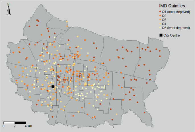

  

  Residents’ Committees in Shijiazhuang by Index of Multiple Deprivation

  Figure 14.3 confirms this, displaying statistically significant clusters of local spatial autocorrelation, measured by local Morans I. This map shows a large cluster of deprived RCs on the city's eastern edge with a smaller cluster on the northwest fringe. The largest cluster of areas with low deprivation can be found to the southeast of the city centre with smaller clusters nearer to the city centre. This is consistent with previous studies demonstrating that more deprived areas are usually situated in the suburbs of Chinese cities (Yuan and Wu 2014). Figure 3 also shows that in most parts of the city, the measure of local spatial autocorrelation is small and not statistically significant suggesting no strong spatial patterning of deprivation. In other words, in most of the city an RC is likely to be surrounded by RCs with varying levels of deprivation.

  Fig. 14.3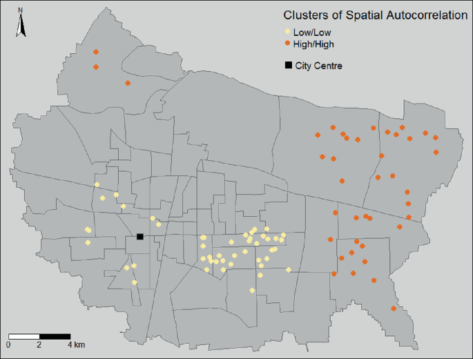

  

  Statistically Significant (p < 0.05) clusters of spatial autocorrelation

• (b) Centralisation

  The DCI for the whole city area is negative and statistically significant (−0.14), meaning that deprived places are on average situated further from the city centre than affluent places, consistent with our findings above. As with all single number segregation measures, this global DCI measure hides the information about the distribution of different groups throughout the city. For example, if there were high concentrations of deprived areas in the centre of the city, low concentrations in the areas surrounding the centre and then high concentrations again at the edge, the DCI would imply that deprived areas were evenly distributed with respect to the centre of the city. This would be somewhat misleading. For this reason, we explore how the DCI changes depending on the number of nearest RCs to the centre that is included in the calculation, adopting an approach proposed by Folch and Rey (2016).

  To do this, after calculating the DCI for the whole dataset, we remove the furthest RC from the centre and recalculate the DCI. We then remove the next furthest RC from the dataset and calculate the DCI a third time. We keep repeating this process until only the two closest RCs to the centre remain. It is then possible to plot how the DCI changes with distance from the city centre as in Fig. 14.4, giving a more in-depth picture of how different groups located throughout the city. This also allows us to test the sensitivity of the DCI to differences in the boundary of the study area. Although selected to approximate the extent of the city's urban area, it is based on administrative areas rather than an in-depth study of the actual city limits.

  Fig. 14.4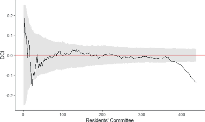

  

  Deprivation Centralisation Index for number of Residents’ Committees away from the centre included. (Grey shaded area—95% confidence intervals from simulation)

  Figure 14.4 shows that the value of the DCI is sensitive to where the city boundaries are drawn. If the furthest ~ 50 RCs were removed from the analysis, the conclusion would be that there is no relationship between deprivation and the city centre. This makes sense when referring back to the map of deprivation in Fig. 14.2. This map clearly shows that the largest area of deprivation is on the periphery to the east of the city; however, there appears to be no clear relationship between deprivation and distance from the centre.

• (c) Typologies of Deprivation.

  To explore the existence of different neighbourhood typologies, we first investigate the similarities and differences in the spatial patterns for each domain. Figure 14.5 shows a map of each domain separately. The spatial patterns for some of the domains appear fairly similar, however, there are some clear and notable differences. In particular, while income and education deprivation is high in the east of the city, employment deprivation in this area is low. The correlations between the domains displayed in Table 14.2 provide support for these preliminary visual observations. There are weak to moderate positive correlations between most of the domains apart from the employment domain, which appears to be uncorrelated with any of the others. The strongest correlation is between the income and education domain.

  Fig. 14.5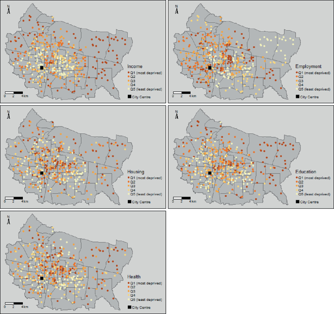

  

  Residents’ Committees in Shijiazhuang, with each IMD domain, plotted separately

  Table 14.2 Correlations between the different IMD domains

  In general, these inter-domain correlations are weak when compared with the correlations between the domains in IMDs for other countries. For example, the correlations between the domains in the South African indices of deprivation range from 0.6 to 0.9 (Noble et al. 2010), while for the English IMD the correlations are typically above 0.8 for the major domains (Ministry for Housing Communities and Local Government 2020). This suggests that there are fewer areas experiencing multiple deprivations in Shijiazhuang compared with the study areas for these other indices. Note that our study area only includes the urban built-up areas and that rural areas of the Shijiazhuang city region are excluded. From looking at the maps for each domain and the correlations between the domains, it is clear that the pattern of deprivation is complex and that it is not simply the case that there are deprived areas that score high on all the domains and affluent areas that score low on all the domains. There appear to be some RCs which have particularly high IMD scores but are deprived in different ways to other RCs which have similarly high scores. In order to learn more about the distribution of deprivation within the city we therefore use the latent class analysis to explore whether there are any underlying groupings of RCs which suffer from similar combinations of deprivations.

  The results of this analysis suggest that there is an affluent or non-deprived class and two distinct deprived classes with different combinations of deprivation factors. The affluent class comprises half of the RCs. This is the least deprived class on all of the indicators, with an average IMD rank of 350, where a rank of 1 denotes the most deprived RC and 450 the least deprived. As we are interested in deprivation rather than affluence, we will not focus upon it further.

  With the lowest average IMD rank (52), the most deprived class comprises 12% of the total RCs. RCs in this class have the highest levels of income deprivation, with particularly high proportions of industrial workers, though low proportions of low-skilled service sector workers. 88% of RCs in this class are in the highest two quintiles for industrial workers, whereas 98% of the RCs are in the lowest two quintiles for low-skilled service sector workers. For this reason, we name it the ‘industrial deprived class.’ RCs in this class also have the highest levels of health and education deprivation, with 95% and 71% of them in the most deprived two quintiles for these two domains, respectively. On the other hand, they have low employment deprivation, with 81% of RCs in the least deprived two quintiles. In terms of the housing domain, the areas have high household amenity deprivation, with 100% of RCs in this class in the most deprived two quintiles, but at the same time low levels of overcrowding, for which 79% of RCs in this class are in the least deprived two quintiles.

  The final class, consisting of 37% of all RCs, is also deprived but slightly less so. The average IMD rank in this class is 82. RCs in this class are deprived in terms of income, though they have low levels of industrial workers (only 27% of RCs in this class are in the top two quintiles). Instead, they have the highest levels of low-skilled service sector workers with 78% of RCs in this class in the top two quintiles for this occupation. We, therefore, name these areas ‘low-skilled service deprived.’ The level of education and health deprivation of the RCs in this class is mixed but tends to be higher rather than lower. Some 45% and 48%, respectively, of RCs are in the top two quintiles of deprivation for these domains. RCs in this class have the highest levels of employment deprivation and the worst levels of overcrowding with 51% and 54% in the most deprived two quintiles for these two indicators. They also tend to be deprived in terms of housing amenities with 61% of RCs in the most deprived two quintiles. Interestingly although not included in the LCA, further exploration shows that this class of RCs has by far the highest proportion of rural migrants without urban hukou status.²

  Figure 14.6 maps the RCs in each of the three classes and shows a clear pattern across the city. This map shows that the RCs in the industrial deprived class are highly clustered and can be found exclusively on the periphery of the city, mainly in the sub-districts on the eastern fringe. On the other hand, the RCs in the low-skilled service deprived class tend to be found closer to the city centre, although their geographical distribution is more variable across the city. Table 14.3 summarises the differences between the RCs in the two classes with different deprivation profiles.

  Fig. 14.6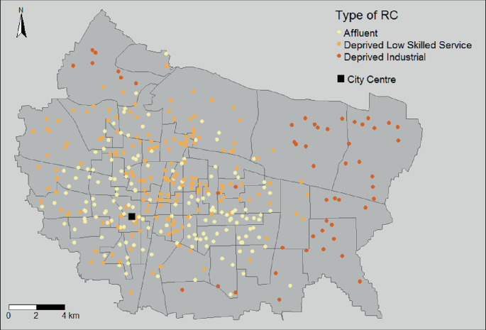

  

  Map of the three types of Residents’ Committee

  Table 14.3 The two types of deprived Residents’ Committees compared

4 Conclusion

In this paper, we have outlined a general method for producing an Index of Multiple Deprivation in China. We have shown the importance of drawing upon the theoretical background of deprivation when calculating deprivation indices and have therefore been able to build upon previous attempts to measure deprivation using Chinese census data. Using data from the city of Shijiazhuang in Hebei Province, we have employed our method to produce an IMD for the city and then used the results to provide a deeper understanding of deprivation within a medium-sized Chinese city.

The most important substantive finding from this analysis is the complex spatial nature of multiple deprivations in Shijiazhuang. The latent class analysis has shown that there are different types of deprived areas that experience different deprivation profiles and that these areas are to be found in different parts of the city. While the more traditional forms of deprived areas with poor household amenities, low education and low incomes still exist, a more modern type of deprived area, with high levels of unemployment and household overcrowding, has emerged in pockets of Shijiazhuang. While they did not explore different types of deprivation, this reflects the analysis of Yuan et al. (2018) in Guangzhou who found an increase in urban deprivation relative to rural areas between 2000 and 2010. This is likely to be explained by growth in this second type of deprivation. This also fits with other reports of new forms of deprivation in urban environments that have emerged after rapid urban expansion. The benefits of rapid economic growth in China have not been shared equally (Wu 2004; Ouyang et al. 2017). Different policy responses are therefore important to address areas with varying deprivation profiles. This finding also highlights the importance of an approach to measuring deprivation that measures different domains of deprivation separately, as a single measure would hide this underlying complexity. To take this further, future research should look for similar patterns of deprivation in cities of varying sizes and also whether there were different groupings of deprivations in rural as opposed to urban areas. Additionally, understanding the link between new kinds of deprivation and migrant settlement patterns, particularly with respect to urban villages, is important (Hao et al. 2013).

The greatest obstacle to calculating deprivation indices in China is the data. For example, the indicators for some of the domains in this study are only available at a coarser scale than our unit of analysis. Moreover, some of the indicators are fairly crude measures of the underlying concept. Further research could conduct some form of ground truthing—direct observation of living conditions for a selection of neighbourhoods—to test the validity of the deprivation indicators. These issues are unlikely to affect our understanding of the overall spatial patterns of deprivation within the city. However, measurement error becomes potentially very important if the goal is to use scores for apportioning funding to the most deprived RCs. While this ultimately represents a limitation within our study, it also highlights the importance of the statistical procedures we have outlined, which minimise measurement error as far as is practicably possible.

One option for future research is to combine other data sources alongside the census data such as administrative data (as in the case of the English IMD), survey data, or other types of geographical data. For example, Chen and Yeh (2018) have recently used points of interest and road network data to develop a measure of accessibility to services for different areas of Guangzhou. A method like this can potentially be adapted to create an ‘accessibility to services’ domain. Another possible avenue for future research is to develop a more robust weighting system for combining the domains. By working with potential end-users of the data it would be possible to determine the criteria for more accurately weighting indicative levels of deprivation in China.

In conclusion, while analysing deprivation in China is not easy, we have outlined a framework using reliable statistical techniques based on the English Indices of Deprivation, which can create deprivation indices in China. This framework provides opportunities to improve understanding of the socio-spatial nature of deprivation in Chinese cities as well as being a potential useful tool for policy makers.

References

Anselin L (1995) Local indicators of spatial association—LISA. Geogr Anal 27(2):93–115. https://doi.org/10.1111/j.1538-4632.1995.tb00338.x
Bailey N et al (2018) Reconsidering the relationship between air pollution and deprivation. Int J Environ Res Public Health. https://doi.org/10.3390/ijerph15040629
Carstairs V, Morris R (1989) Deprivation: explaining differences in mortality between Scotland and England and Wales. BMJ. https://doi.org/10.1136/bmj.299.6704.886
Chen Z, Yeh AG-O (2018) Accessibility inequality and income disparity in urban china: a case study of Guangzhou. Ann Am Assoc Geogr 1–21
Folch DC, Rey SJ (2016) The centralization index: a measure of local spatial segregation. Pap Regnal Sci 95(3):555–576 https://doi.org/10.1111/pirs.12145
Galster G, Sharkey P (2017) Spatial foundations of inequality: a conceptual model and empirical overview. RSF: Russell Sage Found J Soc Sci 3(2):1–33. https://doi.org/10.7758/rsf.2017.3.2.01
Han J, Guo H, Zhang M (2016) China’s “New Normal” and Its Quality of Development. In: Proceedings of the 2nd Czech-China scientific conference 2016, pp 175–188
Hao P et al (2013) What drives the spatial development of urban villages in China? Urban Stud 50(16):3394–3411. https://doi.org/10.1177/0042098013484534
He S, Li SM, Chan KW (2015) Migration, communities, and segregation in Chinese cities: Introducing the special issue. Eurasian Geogr Econ. https://doi.org/10.1080/15387216.2015.1103661
Langlois A, Kitchen P (2001) Identifying and measuring dimensions of urban deprivation in Montreal: an analysis of the 1996 census data. Urban Stud. https://doi.org/10.1080/00420980020014848
Linzer D, Lewis J (2016) ‘Package “poLCA”’. https://cran.r-project.org/web/packages/poLCA/poLCA.pdf
Ministry for Housing Communities and Local Government (2020) ‘English indices of deprivation 2019’. Author’s calculation from data. https://www.gov.uk/government/statistics/english-indices-of-deprivation-2019
Noble M et al (2006) Measuring multiple deprivation at the small-area level. Environ Plan A. https://doi.org/10.1068/a37168
Noble M et al (2010) Small area indices of multiple deprivation in South Africa. Soc Indic Res. https://doi.org/10.1007/s11205-009-9460-7
Ouyang W et al (2017) Spatial deprivation of urban public services in migrant enclaves under the context of a rapidly urbanizing China: an evaluation based on suburban Shanghai. Cities. https://doi.org/10.1016/j.cities.2016.06.004
Pampalon R, Raymond G (2000) A deprivation index for health and welfare planning in Quebec. Chronic Dis Can. https://doi.org/10.1172/JCI200422053
Rae A (2012) Spatially concentrated deprivation in england: an empirical assessment. Regnal Stud 46(9):1183–1199. https://doi.org/10.1080/00343404.2011.565321
Salmond C (1998) NZDep91: a New Zealand index of deprivation. Aust N Z J Public Health. https://doi.org/10.1111/j.1467-842X.1998.tb01505.x
Tammaru T et al (2018) Relationship between income inequality and residential segregation of socioeconomic groups. Regnal Stud 1–12
Townsend P (1987) Deprivation*. J Soc Policy 16(2):125–146
Townsend P, Davidson N (1988) Health and deprivation: inequalities and the north. Stat Med
Weng M et al (2017) Area deprivation and liver cancer prevalence in shenzhen, China: a spatial approach based on social indicators. Soc Indic Res. https://doi.org/10.1007/s11205-016-1358-6
Wu F (2004) Urban poverty and marginalization under market transition: the case of Chinese cities. Int J Urban Reg Res. https://doi.org/10.1111/j.0309-1317.2004.00526.x
Wu Q et al (2014) Socio-spatial differentiation and residential segregation in the Chinese city based on the 2000 community-level census data: a case study of the inner city of Nanjing. Cities. https://doi.org/10.1016/j.cities.2014.02.011
Yang S, Wang MYL, Wang C (2015) Socio-spatial restructuring in Shanghai: sorting out where you live by affordability and social status. Cities. https://doi.org/10.1016/j.cities.2014.12.008
Yuan Y et al (2018) Exploring urban-rural disparity of the multiple deprivation index in Guangzhou City from 2000 to 2010. Cities. https://doi.org/10.1016/j.cities.2018.02.016
Yuan Y, Wu F (2014) ‘The development of the index of multiple deprivations from small-area population census in the city of Guangzhou. PRC’ Habitat Int. https://doi.org/10.1016/j.habitatint.2013.07.010
Yuan Y, Wu F, Xu X (2011) Multiple deprivations in transitional chinese cities: a case study of guangzhou. Urban Aff Rev. https://doi.org/10.1177/1078087411400370
Zhang ML, Pryce G (2019) The dynamics of poverty, employment and access to amenities in polycentric cities: measuring the decentralisation of poverty and its impacts in England and Wales. Urban Stud
Zhao P (2013) The impact of urban sprawl on social segregation in Beijing and a Limited Role for Spatial Planning. Tijdschr Voor Econ En Soc Geogr 104(5):571–587. https://doi.org/10.1111/tesg.12030
Acknowledgements
This research was funded by the Economic and Social Research Council (ESRC) through the ‘Global Challenges Research Fund: Dynamics of Health & Environmental Inequalities in Hebei Province, China’ project (Grant Reference: ES/P003567/1), and the ‘Understanding Inequalities’ project (Grant Reference ES/P009301/1).
Author information
Authors and Affiliations
Corresponding author
Editor information
Editors and Affiliations
Rights and permissions
Open Access This chapter is licensed under the terms of the Creative Commons Attribution 4.0 International License (http://creativecommons.org/licenses/by/4.0/), which permits use, sharing, adaptation, distribution and reproduction in any medium or format, as long as you give appropriate credit to the original author(s) and the source, provide a link to the Creative Commons license and indicate if changes were made.
The images or other third party material in this chapter are included in the chapter's Creative Commons license, unless indicated otherwise in a credit line to the material. If material is not included in the chapter's Creative Commons license and your intended use is not permitted by statutory regulation or exceeds the permitted use, you will need to obtain permission directly from the copyright holder.
Copyright information
© 2021 The Author(s)
About this chapter
Cite this chapter
Owen, G., Chen, Y., Pryce, G., Birabi, T., Song, H., Wang, B. (2021). Deprivation Indices in China: Establishing Principles for Application and Interpretation. In: Pryce, G., Wang, Y.P., Chen, Y., Shan, J., Wei, H. (eds) Urban Inequality and Segregation in Europe and China. The Urban Book Series. Springer, Cham. https://doi.org/10.1007/978-3-030-74544-8_14
Download citation
DOI: https://doi.org/10.1007/978-3-030-74544-8_14
Published:
Publisher Name: Springer, Cham
Print ISBN: 978-3-030-74543-1
Online ISBN: 978-3-030-74544-8
eBook Packages: HistoryHistory (R0)