
Abstract
In this chapter, we will elaborate on our rationale for presenting yet another approach to well-posedness of partial differential equations. In particular, we will highlight conceptual differences between well established rationales and the one presented here. To start with, let us consider why we avoid the usual prominent role of the Laplacian in mathematical physics.
Access this chapter
Tax calculation will be finalised at checkout
Purchases are for personal use only
Notes
- 1.
Recall that for a closed operator A, we always consider \(\operatorname {dom}\left (A\right )\) as a Hilbert space with respect to its graph inner product . Thus, as Hilbert spaces \(\operatorname {dom}\left (A\right )\) and \(\operatorname {dom}\left (B\right )\) maybe different, whereas as sets they can be equal!
- 2.
We have not encountered any other authors, who use this kind of set-up, being aware of the skew-selfadjointness of the underlying spatial operator A.
- 3.
Another way of expressing the Eqs. (3.2.2) and (3.2.3), would be to write
$$\displaystyle \begin{aligned} \left(\partial_{0}+A\right)G=\delta \end{aligned}$$or if we wished to avoid introducing the Dirac-δ-distribution and to establish the idea of operators as solutions:
$$\displaystyle \begin{aligned} \partial_{0}\left(G\left(\:\cdot\:\right)u_{0}-\chi_{\mathbb{R}_{>0}}u_{0}\right)+AG\left(\:\cdot\:\right)u_{0}=0 \end{aligned}$$for \(u_{0}\in \operatorname {dom}\left (A\right )\). Note that
$$\displaystyle \begin{aligned} G\left(\:\cdot\:\right)u_{0}-\chi_{\mathbb{R}_{>0}}u_{0}=\left(\chi_{\mathbb{R}_{>0}}U\left(\:\cdot\:\right)\right)u_{0}-\chi_{\mathbb{R}_{>0}}u_{0} \end{aligned}$$has no jump at the origin and indeed a (weak) time derivative in \(H_{\varrho ,0}\left (\mathbb {R};H\right )\), which is \(G\left (\:\cdot \:\right )Au_{0}=AG\left (\:\cdot \:\right )u_{0}\).
- 4.
This may not be the “energy balance ” that the reader may recall (for example for acoustic waves) . Let us assume that M 1 = 0. Then (3.2.5) is just stating that
$$\displaystyle \begin{aligned} \frac{1}{2}\left\langle u|u\right\rangle _{H}=\frac{1}{2}\left|u\right|{}_{H}^{2} \end{aligned}$$is constant in time on \(\left [0,\infty \right [\). In terms of the group generated by A this is to say that
$$\displaystyle \begin{aligned} t\mapsto\frac{1}{2}\left|u\right|{}_{H}^{2}\left(t\right)=\frac{1}{2}\left|\exp\left(-tA\right)u_{0}\right|{}_{H}^{2} \end{aligned}$$is a constant function, which is of course a feature of the group elements being unitary , and the constant is \(\frac {1}{2}\left |u_{0}\right |{ }_{H}^{2}\). Further, since \(\exp \left (-tA\right )\) commutes with any other (Borel) function f of \(\frac {1}{\mathrm {i}}A\) in the sense of spectral theory,
$$\displaystyle \begin{aligned} \left[0,\infty \right[\ni t\mapsto\frac{1}{2}\left|f\left(\frac{1}{\mathrm{i}}A\right)\exp\left(-tA\right)u_{0}\right|{}_{H}^{2}=\frac{1}{2}\left|\exp\left(-tA\right)f\left(\frac{1}{\mathrm{i}}A\right)u_{0}\right|{}_{H}^{2}=\frac{1}{2}\left|f\left(\frac{1}{\mathrm{i}}A\right)u_{0}\right|{}_{H}^{2} \end{aligned}$$is also a constant function for all \(u_{0}\in \operatorname {dom}\left (f\left (\frac {1}{\mathrm {i}}A\right )\right )\). In particular, assuming that f is the identity on \(\mathbb {R}\) and \(u_{0}\in \operatorname {dom}\left (A\right )\), we get
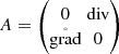
$$\displaystyle \begin{aligned} t\mapsto\frac{1}{2}\left|\frac{1}{\mathrm{i}}Au\left(t\right)\right|{}_{H}^{2}=\frac{1}{2}\left|Au\left(t\right)\right|{}_{H}^{2}=\frac{1}{2}\left|Au_{0}\right|{}_{H}^{2} \end{aligned}$$on \(\left [0,\infty \right [\). In our current example, (3.1.9) with α 0 = 1, μ = 1 and α ∗ = 0,
 and so
for \(t\in \left [0,\infty \right [\). From the first equation of (3.1.9) we know that \(\partial _{0}p=-\operatorname {div} v\) on \(\left ]0,\infty \right [\). Thus,
 (3.2.4)
for \(t\in \left ]0,\infty \right [\). By the continuity properties of the group generated by A, (3.2.4) also holds for t = 0 so that

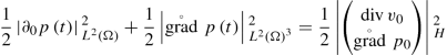
for \(t\in \left [0,\infty \right [\), which is the more common form of energy conservation in the context of acoustic waves as the sum of “kinetic energy ” \(\frac {1}{2}\left |\partial _{0}p\left (t\right )\right |{ }_{L^{2}\left (\Omega \right )}^{2}\) and “potential energy ”
 .
. - 5.
There is a well-developed theory for sums of unbounded operators, see e.g. [7, 10]. The criteria are, however, not easily manageable and go far beyond the complexity of our simple setup. In hindsight, it seems indeed rather wasteful and misleading to further the impression that considerations of such sophistication are needed to understand the standard evolutionary problems of engineering and mathematical physics.
The dramatic simplification in our setup is due to the strict positive definiteness of ∂ 0, to the skew-selfadjointness of A and the fact that ∂ 0 and A commute.
- 6.
If we had considered second order in time equations, then the numerical range condition is more involved. Indeed, note that
$$\displaystyle \begin{aligned} \begin{array}{rcl} \partial_{0}^{2} &\displaystyle = &\displaystyle \left(\left(\partial_{0}-\varrho\right)+\varrho\right)^{2}\\ &\displaystyle = &\displaystyle \varrho^{2}+\left(\partial_{0}-\varrho\right)^{2}+2\varrho\left(\partial_{0}-\varrho\right) \end{array} \end{aligned} $$and so, since ∂ 0 − ϱ is skew-selfadjoint ,
$$\displaystyle \begin{aligned} \begin{array}{rcl} \operatorname{\mathfrak{Re}}\partial_{0}^{2} &\displaystyle = &\displaystyle \varrho^{2}+\left(\partial_{0}-\varrho\right)^{2}\\ &\displaystyle = &\displaystyle \varrho^{2}-\left(\frac{1}{\mathrm{i}}\left(\partial_{0}-\varrho\right)\right)^{2},\\ \operatorname{\mathfrak{Im}}\partial_{0}^{2} &\displaystyle = &\displaystyle 2\varrho\frac{1}{\mathrm{i}}\left(\partial_{0}-\varrho\right). \end{array} \end{aligned} $$Since the spectrum \(\sigma \left (\frac {1}{\mathrm {i}}\left (\partial _{0}-\varrho \right )\right )\) is all of \(\mathbb {R}\) we get
$$\displaystyle \begin{aligned} \begin{array}{rcl} w\left(\partial_{0}^{2}\right)=\sigma\left(\partial_{0}^{2}\right) &\displaystyle = &\displaystyle \left\{ \varrho^{2}-r^{2}+\mathrm{i}2\varrho r|\,r\in\mathbb{R}\right\} \\ &\displaystyle = &\displaystyle \left\{ \varrho^{2}-\frac{1}{4}\varrho^{-2}s^{2}+\mathrm{i} s|\,s\in\mathbb{R}\right\} , \end{array} \end{aligned} $$which is a parabola opening to the left, symmetric around the real axis, based at ϱ 2.
- 7.
This construction can be lifted to the higher dimensional situation provided Ω has the appropriate symmetry properties.
- 8.
Introducing a skew-selfadjoint spatial operator is not just an interesting “trick”. In the spirit of footnote 2, this way we get an energy balance law for any solution
 .
. - 9.
Some will find it a good solution of the problem to look for another door, which is really locked, to deploy their door-breaking skills there instead!
 and so


 .
. .
.References
W. Arendt, C.J.K. Batty, M. Hieber, F. Neubrander, Vector-Valued Laplace Transforms and Cauchy Problems. Monographs in Mathematics, vol. 96 (Birkhäuser, Basel, 2001), xi, 523 p.
C. Batty, L. Paunonen, D. Seifert, Optimal energy decay in a one-dimensional coupled wave-heat system. J. Evol. Eq. 16(3), 649–664 (2016)
H. Brézis, A. Haraux, Image d’une somme d’opérateurs monotones et applications. Isr. J. Math. 23, 165–186 (1976)
G. Da Prato, P. Grisvard, Sommes d’operateurs lineaires et equations differentielles operationnelles. J. Math. Pures et Appl. 54, 305–387 (1975)
K. Engel, R. Nagel, One-Parameter Semigroups for Evolution Equations, vol. 194 (Springer, New York, 1999)
S. Franz, M. Waurick, Resolvent estimates and numerical implementation for the homogenisation of one-dimensional periodic mixed type problems. Z. Angew. Math. Mech. 98(7), 1284–1294 (2018)
S. Franz, S. Trostorff, M. Waurick, Numerical methods for changing type systems. Technical report. IMA J. Numer. Anal. 39(2), 1009–1038 (2019)
E. Hille, R.S. Phillips, Functional Analysis and Semigroups. American Mathematical Society Colloquium Publications, vol. 31 (American Mathematical Society, Providence, 1957)
R. Picard, S. Trostorff, M. Waurick, M. Wehowski, On non-autonomous evolutionary problems. J. Evol. Eq. 13(4), 751–776 (2013)
R. Picard, S. Seidler, S. Trostorff, M. Waurick, On abstract grad-div systems. J. Differ. Eq. 260(6), 4888–4917 (2016)
R. Picard, S. Trostorff, M. Waurick, On a comprehensive class of linear control problems. IMA J. Math. Control Inf. 33(2), 257–291 (2016)
A.F.M. ter Elst, G. Gorden, M. Waurick, The Dirichlet-to-Neumann operator for divergence form problems. Annali di Matematica Pura ed Applicata, 198(1): 177–203, (2019)
S. Trostorff, A characterization of boundary conditions yielding maximal monotone operators. J. Funct. Anal. 267(8), 2787–2822 (2014)
S. Trostorff, Exponential stability and initial value problems for evolutionary equations. Habilitation, TU Dresden, 2018
M. Waurick, Stabilization via homogenization. Appl. Math. Lett. 60, 101–107 (2016)
Author information
Authors and Affiliations
Rights and permissions
Copyright information
© 2020 Springer Nature Switzerland AG
About this chapter

Cite this chapter
Picard, R., McGhee, D., Trostorff, S., Waurick, M. (2020). But What About the Main Stream?. In: A Primer for a Secret Shortcut to PDEs of Mathematical Physics. Frontiers in Mathematics. Birkhäuser, Cham. https://doi.org/10.1007/978-3-030-47333-4_3
Download citation
DOI: https://doi.org/10.1007/978-3-030-47333-4_3
Published:
Publisher Name: Birkhäuser, Cham
Print ISBN: 978-3-030-47332-7
Online ISBN: 978-3-030-47333-4
eBook Packages: Mathematics and StatisticsMathematics and Statistics (R0)