PAKEs: New Framework, New Techniques and More Efficient Lattice-Based Constructions in the Standard Model

Abstract

Password-based authenticated key exchange (PAKE) allows two parties with a shared password to agree on a session key. In the last decade, the design of PAKE protocols from lattice assumptions has attracted lots of attention. However, existing solutions in the standard model do not have appealing efficiency. In this work, we first introduce a new PAKE framework. We then provide two realizations in the standard model, under the Learning With Errors (LWE) and Ring-LWE assumptions, respectively. Our protocols are much more efficient than previous proposals, thanks to three novel technical ingredients that may be of independent interests. The first ingredient consists of two approximate smooth projective hash (ASPH) functions from LWE, as well as two ASPHs from Ring-LWE. The latter are the first ring-based constructions in the literature, one of which only has a quasi-linear runtime while its function value contains $\varTheta (n)$ field elements (where n is the degree of the polynomial defining the ring). The second ingredient is a new key conciliation scheme that is approximately rate-optimal and that leads to a very efficient key derivation for PAKE protocols. The third one is a new authentication code that allows to verify a MAC with a noisy key.

1 Introduction

Key exchange is a fundamental and widely used cryptographic mechanism allowing two parties to securely share a session key over a public unreliable channel. In its original form, suggested in the seminal work of Diffie and Hellman, key exchange does not provide authentication and security against an active adversary who has full control of the communication channel. Authenticated key exchange additionally allows each user to authenticate identities of others using either Public-key Infrastructure (PKI) such as TLS/SSL and IKE, or some pre-shared information. The pre-shared information can be either a high-entropy cryptographic key or a low-entropy password. In practice, the latter is more convenient for human users who have limited memory. The study of password authenticated key exchange (PAKE) was initiated by Bellovin and Merritt [4]. A secure PAKE protocol must resist offline dictionary attacks, in which the adversary attempts to determine the password using information from previous executions.

Related Work. Since the pioneering work of Bellovin and Merritt [4] in 1992, PAKE has been extensively studied. The first provably secure PAKE protocol was suggested in [3], but its security analysis resorts to the random oracle model (ROM). Goldreich and Lindell [13] then introduced the first construction without ROM, based on general assumptions. A reasonably efficient protocol was put forward by Katz, Ostrovsky and Yung [17], which was later abstracted by Gennaro and Lindell [11] into a framework based on smooth projective hash (SPH) functions. However, these protocols did not support mutual authentication (MA). That is, the participant cannot make sure that the party he is interacting with, is the right person. Of course, one can make it up with additional flows, but this will increase the round complexity. Jiang and Gong (JG) [16] then proposed a more efficient protocol with MA without increasing round complexity.

In this work, we are interested in PAKE protocols from lattices. The first protocol was introduced in 2009 by Katz and Vaikuntanathan (KV) [18], whose main ideas are as follows. Alice and Bob first send a CCA-secure ciphertext to each other. Then, they try to compute approximate smooth projective hashing (ASPH) values on the ciphertexts and conduct a key reconciliation to derive a session key. Their key reconciliation mechanism consists of two steps: the first step aims to extract a bit from the ASPH value which is slightly noisy, while the second step is dedicated to correct the error using error-correcting code (ECC). This mechanism is relatively inefficient as it can extract at most one bit per field element. Furthermore, the underlying CCA-secure ciphertext (hence the ASPH) is quite costly, as it includes $\omega (\log n)$ CPA-secure ciphertexts¹.

Groce and Katz (GK) [15] abstracted the JG protocol [16] into a framework for PAKE, yielding a more efficient lattice-based protocol than KV. The idea of the GK framework is as follows. Alice sends a CPA-secure encryption C of password $\pi$ to Bob. Bob then computes an SPH value h on $(\pi , C)$. Then, they conduct authentication via a CCA-secure encryption with randomness determined by h. This framework can be adapted into the ASPH setting using KV’s ASPH with their two-step key reconciliation. A realization was given by Benhamouda et al. [5]. Canetti et al. [6] demonstrated another framework for obtaining PAKE (without ASPH), via oblivious transfer (OT). They use OT to transfer $L'$ bits for each password bit and finally achieve the authentication via the CCA-secure encryption approach [15, 16].

Zhang and Yu [28] proposed a PAKE framework from a new ASPH built on a “splittable CCA-secure encryption”. However, their realization is in the ROM. Another ROM-based PAKE protocol from lattices is due to Ding et al. [8]. In this work, we only study PAKE protocols without the ROM.

Thus, all existing PAKE frameworks have certain efficiency issues, and do not admit efficient lattice-based realizations in the standard model. Moreover, a CCA-secure encryption seems to be an essential ingredient in them. This raises two interesting questions: (1) From a theoretical point of view, is it possible to achieve a secure PAKE without relying on any CCA-secure encryption or its variant? (2) From a more practical point of view, how to design lattice-based PAKEs in the standard model with better efficiency than previous ones? Tackling these questions would likely require new technical insights.

Our Contributions and Techniques. In this work, we answer the above two questions in the affirmative. Our contributions are threefold. First, we put forward a new framework for obtaining secure PAKE protocols that does not require any CCA-secure encryption or its variant. Second, we introduce several new technical building blocks, that enable efficient standard-model instantiations of our framework in general, and from lattices - in particular. Third, we explicitly give two realizations of our framework, based on the plain Learning With Errors (LWE) and the Ring-LWE assumptions, which enjoy security guarantees from worst-case problems in general lattices [26] and ideal lattices [19], respectively. Our PAKEs compare very favourably with previous lattice-based protocols in the standard model. We also provide implementation results of the Ring-LWE-based scheme to demonstrate its practical feasibility. To the best of our knowledge, this is the first implementation of any lattice-based PAKE in the standard model, and the performance is quite encouraging.

New PAKE Framework. Let us first discuss the high-level ideas of our new PAKE framework. It relies on an ASPH, a key reconciliation scheme and a new notion of key-fuzzy message authentication code (KF-MAC). KF-MAC allows the verification key to be slightly different from the original authentication key. We define a generic ASPH on top of a commitment scheme. Given secret k, input $\pi$ and a value y in the commitment space (not necessarily a commitment to $\pi$), an ASPH function $\mathcal{H}$ computes the hash value $\mathcal{H}(k, \pi , y).$ If y is indeed a commitment to $\pi$ with witness $\tau$, then $\mathcal{H}(k, \pi , y)$ can also be approximated by an alternative function $\hat{\mathcal{H}}$ as $\hat{\mathcal{H}}(\tau , \alpha (k))$, where $\alpha (k)$ is called the projection key of k. The important property for ASPH is smoothness: if y is a commitment to $\pi ' (\ne \pi )$, then $(\mathcal{H}(k, \pi , y), \alpha (k))$ are jointly random. We describe our PAKE framework using this generic ASPH. However, to prove the framework security, additional properties on ASPH (which will be clarified later) are required. Our PAKE framework is an integration of three basic processes below.

• Basic key exchange. Alice and Bob use ASPH $(\mathcal{H}_1, \hat{\mathcal{H}}_1, \alpha _1)$ to obtain close secrets.

  • 1. Bob (initiator) first generates a commitment y (with witness $\tau _1$) to password $\pi$. He then sends y to Alice.

  • 2. Upon receiving y, Alice samples a secret k, computes and sends a projection key $\alpha _1(k)$ to Bob. She also computes a hash value $\mathcal{H}_1(k, \pi , y)$.

  • 3. Upon receiving $\alpha _1(k)$, Bob computes $\hat{\mathcal{H}}_1(\tau _1, \alpha _1(k))$. Note that the distance between $\mathcal{H}_1(k, \pi , y)$ and $\hat{\mathcal{H}}_1(\tau _1, \alpha _1(k))$ is typically small.

• Key reconciliation. This process enables Alice (with $\mathcal{H}_1(k, \pi , y)$) and Bob (with $\hat{\mathcal{H}}_1(\tau _1, \alpha _1(k))$) to agree on a secret $\xi ,$ via a one-message key reconciliation scheme . If no attack exists, then $\xi$ derived by Alice and Bob will be the same. To assure this, they need to authenticate each other.

• Authentication. This process uses another ASPH $(\mathcal{H}_2, \hat{\mathcal{H}}_2, \alpha _2)$ and a projection key $V=\alpha _2(O)$ (with a hidden key O) as public parameters. Here Alice and Bob will authenticate each other and derive a session key.

  • 1. Alice deterministically computes commitment w (with witness $\tau _2$) on password $\pi$, using randomness determined by $\xi$. Next, she computes KF-MAC $\eta _0$ on traffic using key $\hat{\mathcal{H}}_2(\tau _2, V).$ Finally, she sends $(w, \eta _0)$ to Bob.

  • 2. Bob uses $\xi$ to repeat Alice’s procedure to verify $(w, \eta _0)$ and compute $\tau _2$. Then, he uses $\hat{\mathcal{H}}_2(\tau _2, V)$ to authenticate himself.

We stress that although three procedures are described separately, they can be integrated into a 3-round protocol. The pictorial outline is given in Fig. 1 and a more detailed version is in Fig. 2. For security, we require the commitment for ASPH $(\mathcal{H}_1, \hat{\mathcal{H}}_1, \alpha _1)$ to have a trapdoor property: with a trapdoor (but without witness $\tau _1$), one verifies if y is a commitment of $\pi$. We call this ASPH type-B ASPH. We require ASPH $(\mathcal{H}_2, \hat{\mathcal{H}}_2, \alpha _2)$ to have strong smoothness: if w is a random (i.e., honestly generated) commitment to $\pi$, then $\hat{\mathcal{H}}_2(\tau _2, V)$ is random (given $w, V, \pi$). We call this ASPH type-A ASPH.

At a high level, our main strategy for proving framework security is the sequence of games: modify the protocol gradually so that the messages in the final game contain no password. Firstly, we can modify the protocol so that $\pi$ in y is a dummy password. This is unnoticeable to the attacker by the commitment hiding property. Then, under this revision, y normally does not contain the correct $\pi$. If this is the case (which can be checked by the trapdoor property of type-B ASPH), then, by smoothness of $\mathcal{H}_1$, $\mathcal{H}_1(k, \pi , y)$ is random. This random distribution will propagate to $\xi .$ Thus, on the one hand, w is a random commitment to $\pi$, and so, by the commitment hiding property, we can revise $\pi$ in w to be a dummy password. On the other hand, by strong smoothness of $\hat{\mathcal{H}}_2$, KF-MAC key $\hat{\mathcal{H}}_2(\tau _2, \alpha _2(O))$ looks random to attacker, and hence, the traffic can not be tampered by KF-MAC property. In fact, an attacker can not impersonate Alice successfully either. Indeed, if he modifies Alice’s message only a little, then the KF-MAC will not change and the traffic will not consistent with the KF-MAC tag. If the attacker modifies Alice’s message too much (or even creates a new one), (simulated) Bob will use $\mathcal{H}_2(O, \pi , w)$ to verify the KF-MAC. By smoothness of $\mathcal{H}_2$, he will not succeed unless w contains the password $\pi .$

After modifications, protocol messages have no password. Attacker can succeed beyond trivial attacks only by constructing y or w that contains the correct $\pi$. So he can not succeed better than simply guessing the password.

New Technical Building Blocks. Together with the new framework, we also introduce three new technical ingredients that may be of independent interest.

• (1) We construct a new reconciliation scheme for close secrets in $\mathbb {Z}_q^\mu$ (in Sect. 3.2). Our scheme can extract $\varTheta (\log q)$ per element in $\mathbb {Z}_q$ and is proven asymptotically rate-optimal. It is much more efficient than all the previous two-step schemes [5, 18, 24], where at most one bit per element in $\mathbb {Z}_q$ can be extracted.

• (2) We give an authentication code with a noisy verification key in Sect. 3.3.

• (3) We provide efficient constructions of ASPHs from both plain LWE and Ring-LWE. In each setting, we construct a type-A ASPH and a type-B ASPH. The LWE-based schemes are as follows.

a. Type-A ASPH. For public parameters $\mathbf{B}\in \mathbb {Z}_q^{m\times (n+L)}$ and $\mathbf{g}\in \mathbb {Z}_q^m$ and an m-length error-correcting code $\mathcal{C}$ with k information symbols, the commitment to $\pi$ has the form $\mathbf{w}=\mathbf{B}{} \mathbf{t}+\mathbf{g}\odot \mathcal{C}(\pi )+\mathbf{x}$, where $\odot$ is the coordinate-wise multiplication, $\mathbf{t}$ is uniformly random over $\mathbb {Z}_q^{n+L}$ and $\mathbf{x}$ is a discrete Gaussian over $\mathbb {Z}_q^m$. The commitment witness is $(\mathbf{t}, \mathbf{x})$. For secret key $\mathbf{O}$ - which is a discrete Gaussian over $\mathbb {Z}_q^{m\times L}$, the projection key is $\mathbf{O}^T\mathbf{B}.$ Then, the projective hashing is computed as $\mathcal{H}(\mathbf{O}, \pi , \mathbf{w})=\mathbf{O}^T(\mathbf{w}-\mathbf{g}\odot \mathcal{C}(\pi ))$, while the alternative hashing is defined as $\hat{\mathcal{H}}((\mathbf{t}, \mathbf{x}), \mathbf{O}^T\mathbf{B})=\mathbf{O}^T\mathbf{B}{} \mathbf{t}.$ If $\mathbf{w}$ is a commitment honestly generated as above, then the two hashing values differ by $\mathbf{O}^T\mathbf{x}$ (which is short as $\mathbf{x}$ and $\mathbf{O}$ are short). For the smoothness, if w is a commitment on $\pi '\ne \pi$, then given $\mathbf{O}^T\mathbf{B}$, value $\mathbf{O}^T(\mathbf{w}-\mathbf{g}\odot \mathcal{C}(\pi ))$ is statistically close to uniform over $\mathbb {Z}_q^L$ (see Theorem 2). For strong smoothness, it requires that given $\mathbf{B}{} \mathbf{t}+\mathbf{x}$ and $\mathbf{O}^T\mathbf{B}$, value $\mathbf{O}^T\mathbf{B}{} \mathbf{t}$ looks random. We prove this using hidden-bits lemma in [9].

b. Type-B ASPH. Type B ASPH is similar to Type A ASPH, except it needs to provide a trapdoor property for the commitment. This property is achieved via the trapdoor simulation techniques in [1, 18].

The ASPHs in the ring-LWE setting essentially follow the same strategy as the LWE-based ones. However, the supporting techniques (i.e., hidden-bits lemma, trapdoor simulation and adaptive smoothness theorem) have to be rebuilt. This turns out to be highly non-trivial. Essentially, this is due to the sparseness of matrix representations for ring operations. Consequently, the random arguments for the LWE case are no longer useful. However, this rebuilding work is worth as ring-LWE ASPHs are much more efficient than LWE-based ones. A detailed informal description is presented in Sect. 5.

Efficient Lattice-Based Instantiations of PAKE in the Standard Model. When putting all building blocks together, we obtain PAKE protocols from plain LWE and Ring-LWE that are much more efficient than previous lattice-based constructions in the standard model. Table 1 provides a summary of the comparison. For simplicity, the table only counts the dominating costs.

Table 1. Comparison among lattice-based PAKEs in the standard model. Here, $m=\varOmega (n\log n)$; k is the password length; $L'$ is the key reconciliation output length (since the output is mostly used as a key for a symmetric-key primitive, $L'\ll n$); the cost for client/server is $\sharp$ of multiplications in $\mathbb {Z}_q$; Comm is the message length in $\mathbb {Z}_q$; $\lambda >3$.

We provide the implementation in Sect. 5.5 for our Ring-LWE-based PAKE protocol. In this proof-of-concept implementation, the Number Theory Library (NTL) [27] is employed without further optimization. To agree on a 16-byte session key, the bandwidth from $P_i$ to $P_j$ is about 40 KB and 167 KB from $P_j$ to $P_i$. Generating public parameters requires about 1.31 s, while $P_i$’s and $P_j$’s computations cost about 0.2 s and 0.71 s, respectively. Although the efficiency is (expectedly) not competitive with the ROM protocol from [8], our implementation demonstrates that the technical ingredients introduced in this work do advance the state of the art of lattice-based PAKEs in the standard model and do bring them much closer to practice. But it still needs further improvement toward practical application. This will be our future direction.

Organization. The rest of the paper is organized as follows. In Sect. 2, we provide necessary background on PAKEs and lattices. The technical ideas, technical building blocks and description of our new PAKE framework are presented in Sect. 3. Our LWE-based and Ring-LWE-based instantiations are provided in Sects. 4 and 5, respectively.

Notations. The transposition of matrix $\varGamma$ is denoted by $\varGamma ^T$; [k] denotes set $\{0, \cdots , k-1\}.$ Vectors are column vectors (unless stated otherwise); $v_i$ or $\mathbf{v}[i]$ denotes the ith component of $\mathbf{v}$; $[\mathbf{v}]_1^L$ denotes the sub-vector $(v_1, \cdots , v_L)^T$ of $\mathbf{v}$. Sampling x from set S uniformly at random is denoted by $x \leftarrow S$; A|B is a concatenation of A with B. $\mathbf{negl}: \mathbb {N} \rightarrow \mathbb {R}$ represents a negligible function: $\lim _{n\rightarrow \infty } \mathbf{negl}(n)p(n)=0$ for any polynomial p(n). The statistical distance between $X_1, X_2$ is $\varDelta (X_1, {X_2}):=\frac{1}{2}\sum _x|P_{X_1}(x)-P_{X_2}(x)|$, where $P_X()$ is the probability mass function of X. We say that $X_1$ and $X_2$ are statistically close if $\varDelta (X_1, X_2)$ is negligible. $||\mathbf{x}||$ is the Euclidean norm of $\mathbf{x}$; $||\mathbf{x}||_\infty =\max _i |x_i|$ is the $\ell _\infty$-norm and $\textsf {dist}_\infty (\cdot , \cdot )$ is the distance measure under $\ell _\infty$-norm. $x\mod q$ denotes the residue of $x\in \mathbb {Z}_q$ in $[0, \cdots , q)$ and $(x)_q$ denotes the residue of $x\in \mathbb {Z}_q$ in $[-q/2, q/2)$. The $\odot$ product is defined as $(a_1, \cdots , a_n)\odot (b_1, \cdots , b_n)=(a_1b_1, \cdots , a_nb_n)$. For $\mathbf{v}\in \mathbb {R}^n,$ Diag$(\mathbf{v})$ is the diagonal matrix with $v_i$ as the (i, i)th entry. For $m_1\times n_1$ matrix $\mathbf{A}$ and $m_2\times n_2$ matrix $\mathbf{B}$, the tensor product $\mathbf{A}\otimes \mathbf{B}$ is the $m_1m_2\times n_1n_2$ matrix $(C_{ij})$ in the block format, where block $C_{ij}=a_{ij} \mathbf{B}$ for any $i\in [m_1], j\in [n_1].$ The (column) concatenation of vectors $\mathbf {v}_1, \ldots , \mathbf {v}_t$ is a long vector, denoted by $(\mathbf{v}_1; \mathbf{v}_2; \cdots ; \mathbf{v}_t)$.

2 Preliminaries

2.1 Security Model of PAKE

In this section, we recall a formal model for a password-authenticated key exchange protocol $\varSigma$. This model is mainly adopted from Bellare et al. [3] with a minor revision in [15]. There are n parties $P_1, \cdots , P_n$ in the system and any two parties share a password. We will use the following notations.

• $\mathcal{D}$: This is the password dictionary. For simplicity, we assume that passwords are chosen uniformly from $\mathcal{D}$.

• $\varPi _i^{\ell _i}$: This is the $\ell _i$-th instance of protocol $\varSigma$ executed by party $P_i$. The number $\ell _i$ is used by $P_i$ to distinguish these instances.

• $Flow_d$: This is the d-th message flow in the execution of protocol $\varSigma .$

• $\mathbf{sid}_i^{\ell _i}$: This is the session identifier of $\varPi _i^{\ell _i}.$ It is only for the purpose of security analysis. Intuitively, two instances jointly executing $\varSigma$ should share the same session identifier. The specification is available only if $\varSigma$ is known.

• $\mathbf{pid}_i^{\ell _i}$: This is the party, which $\varPi _i^{\ell _i}$ is interacting with.

• $sk_i^{\ell _i}$: This is the session key derived by $\varPi _i^{\ell _i}$ after successfully executing $\varSigma .$

Partnering. Instances $\varPi _i^{\ell _i}$ and $\varPi _j^{\ell _j}$ are partnered if (1) $\mathbf{pid}_i^{\ell _i}=P_j$ and $\mathbf{pid}_j^{\ell _j}=P_i$; (2) $\mathbf{sid}_i^{\ell _i}=\mathbf{sid}_j^{\ell _j}.$ The partnering is motivated to identify two instances that are jointly executing protocol $\varSigma$.

Adversarial Model. To define security, we have to specify an attacker’s capabilities. Essentially, we wish to capture man-in-the-middle attacks. The protocol is secure if the adversary can not obtain anything about a session key beyond the trivial findings. Formally, the attacks are modelled through oracles that are maintained by a challenger as follows.

• Execute($i, \ell _i, j, \ell _j$): When this oracle is called, it first checks whether $\varPi _i^{\ell _i}$ and $\varPi _j^{\ell _j}$ are fresh. If not, it does nothing; otherwise, a protocol execution between $\varPi _i^{\ell _i}$ and $\varPi _j^{\ell _j}$ takes place. Finally, the transcript is returned. This is an eavesdropping attack.

• Send($d, i, \ell _i, M)$: When this oracle is called, M is sent to $\varPi _i^{\ell _i}$ as $Flow_d$. If $d=0$ or 1, then a new instance $\varPi _i^{\ell _i}$ is created. If $d=0$, then $M=``\text{ ke }, \textsf {pid}_i^{\ell _i}$” is a key exchange request message (from an upper layer program inside $P_i$). In any case, $\varPi _i^{\ell _i}$ acts according to the specification of $\varSigma$.

• Reveal($i, \ell _i$): This oracle call assumes that $\varPi _i^{\ell _i}$ has successfully completed with a session key $sk_i^{\ell _i}$ derived. Under this, $sk_i^{\ell _i}$ is returned.

• Test($i, \ell _i$): This oracle is to test the secrecy of $sk_i^{\ell _i}$. The adversary is only allowed to query it once. Toward this, $\varPi _i^{\ell _i}$ must have successfully completed with $sk_i^{\ell _i}$ derived. Furthermore, $\varPi _i^{\ell _i}$ and its partnered instance (if any) should not have been issued a $\mathbf{Reveal}$ query. Then, it takes $b\leftarrow \{0, 1\}$. If $b=1,$ then $\alpha _1=sk_i^{\ell _i}$ is provided to adversary; otherwise, a random number $\alpha _0$ from the space of the session key is provided. The adversary then tries to output a guess bit $b'$ of b. He is announced for success if $b'=b.$

Correctness. If two partnered instances both accept, they derive the same key.

Adversarial Success. Having specified the adversarial behaviour, we now define its success. This consists of authentication and secrecy.

• $\diamond$ Mutual authentication. We first define the semi-partnering [15]: instances $\varPi _i^{\ell _i}$ and $\varPi _j^{\ell _j}$ are semi-partnered if they are partnered, or, the following conditions hold: (1) $\textsf {sid}_i^{\ell _i}$ and $\textsf {sid}_j^{\ell _j}$ agree except possibly for the final message flow in $\varSigma$; (2) $\mathbf{pid}_i^{\ell _i}=P_j$ and $\mathbf{pid}_j^{\ell _j}=P_i$. This relaxed partnering is defined to rule out the possible trivial attack where an attacker forwards all the messages except the final one. An attacker breaks mutual authentication if some $\varPi _i^{\ell _i}$ with $\mathbf{pid}_i^{\ell _i}=P_j$ has successfully completed the execution of $\varSigma$ with a session key derived while there does not exist a semi-partnered instance $\varPi _j^{\ell _j}$.

• $\diamond$ Secrecy. An adversary succeeds if $b'=b$.

We use random variable $\mathbf{Succ}$ to denote either of the above two success events. Define the advantage of adversary ${\mathcal A}$ as $\mathbf{Adv}$(${\mathcal A}$):= $2\Pr [\mathbf{Succ}]-1.$

Definition 1

A password authenticated key exchange protocol $\varSigma$ is secure if it is correct and for any PPT adversary $\mathcal{A}$ that makes Send queries at most $Q_{s}$ times, it holds that $\mathbf{Adv}({\mathcal A})\le \frac{Q_{s}}{|\mathcal{D}|}+\mathbf{negl}(n).$

2.2 Lattices and Hard Random Lattices

We now give a brief background on lattices. Let $\mathbf{B}=\{\mathbf{b}_1, \cdots , \mathbf{b}_n\}\subset \mathbb {C}^m$ consist of n linearly independent vectors. An m-dimensional lattice with basis $\mathbf{B}$ is defined as $\mathcal{L}(\mathbf{B})=\left\{ \sum _{i=1}^n a_i \mathbf{b}_i\mid {a}_i\in \mathbb {Z}\right\}$. For lattice $\varLambda$, the Euclidean norm of its shortest non-zero vector is denoted by $\lambda _1(\varLambda )$. If we use the $\ell _\infty$-norm, it is denoted by $\lambda ^\infty _1(\varLambda ).$ The dual lattice of $\varLambda \subseteq \mathbb {C}^m$ is defined as $\varLambda ^\vee =\{\mathbf{y}: \langle \mathbf{x}, \bar{\mathbf{y}}\rangle =\sum _{i}x_iy_i\in \mathbb {Z}, \forall \mathbf{x}\in \varLambda \},$ where $\bar{\mathbf{y}}$ is the complex conjugate of $\mathbf{y}$.

For $s>0$ and $\mathbf{x}\in \mathbb {R}^m$, Gaussian function with parameter s is $\rho _{s}(\mathbf{x})=\exp (-\frac{\pi ||\mathbf{x}||^2}{s^2})$. The discrete Gaussian distribution over lattice $\varLambda \subseteq \mathbb {R}^m$ with parameter s is defined as $D_{\varLambda , s}(\mathbf{x})=\frac{\rho _{s}(\mathbf{x})}{\rho _{s}({\varLambda })}, \forall \mathbf{x}\in \varLambda .$

For $m\ge 2$, let $H=\{\mathbf{x}\in \mathbb {C}^{\phi (m)}: x_i=\bar{x}_{m-i}, \forall i\in \mathbb {Z}_m^*\}$, where $x_i$ in $\mathbf{x}\in H$ is indexed by $i\in \mathbb {Z}_m^*$ and $\phi (m)$ is the Euler function. We are interested in lattice $\varLambda \subseteq H$. It is an inner product space over $\mathbb {R}$, isomorphic to $\mathbb {R}^{\phi (m)}$; see [20] for details. Hence, $D_{\varLambda , s}(\mathbf{x})$ with $\varLambda \subset H$ can be defined in exactly the same way as $\varLambda \subseteq \mathbb {R}^n$. Micciancio and Regev [22] defined a quantity smoothing parameter.

Definition 2

For a lattice $\varLambda$ and $\epsilon >0$, the smoothing parameter $\eta _\epsilon (\varLambda )$ is the smallest s so that $\rho _{1/s}(\varLambda ^\vee \backslash \{\mathbf{0}\})\le \epsilon .$

Usually, $\eta _\epsilon (\varLambda )$ is desired to be small. Then, the following result is useful.

Lemma 1

[25] For an m-dimensional lattice $\varLambda$, $\eta _\epsilon (\varLambda )\le \frac{\sqrt{\log (2m/(1+1/\epsilon ))/\pi }}{\lambda ^\infty _1(\varLambda ^\vee )}.$

The following bounds are taken from [22, Lemma 4.4] and [2, Lemma 2.4].

Lemma 2

For $s\ge \omega (\sqrt{\log m})$ and any $\mathbf{v}\in \mathbb {R}^m$ and any $t>0$, if $\mathbf{e}\leftarrow D_{\mathbb {Z}^m, s}$, then $P(||\mathbf{e}||>s\sqrt{m})\le O(2^{-m})$ and $P(|\mathbf{v}^T\mathbf{e}|>st||\mathbf{v}||)\le 2e^{-\pi t^2}$.

Hard Random Lattices. For integers q, m, n and $\mathbf{A}\in \mathbb {Z}_q^{m\times n}$ of rank n, let $\varLambda ^{\perp }(\mathbf{A})=\{\mathbf{e}\in \mathbb {Z}^m\mid \mathbf{e}^T\mathbf{A}=\mathbf{0} \mod q\}$ and $\varLambda (\mathbf{A})=\{\mathbf{y}\in \mathbb {Z}^m\mid \mathbf{y}=\mathbf{A}{} \mathbf{s} \mod q, \mathbf{s}\in \mathbb {Z}^n\}.$ It is easy to verify that $\varLambda ^\perp (\mathbf{A})=q\cdot \left( \varLambda (\mathbf{A})\right) ^\vee$ and $\varLambda (\mathbf{A})=q\cdot \left( \varLambda ^\perp (\mathbf{A})\right) ^\vee$. Here is a useful lemma on $\varLambda ^\perp (\mathbf{A})$.

Lemma 3

[12] If rows of $\mathbf{A}\in \mathbb {Z}_q^{m\times n}$ generate $\mathbb {Z}_q^{1\times n}$ and $r\ge \eta _\epsilon (\varLambda ^\perp (\mathbf{A}))$, then for $\mathbf{e}\leftarrow D_{\mathbb {Z}^m, r}$, $\varDelta (\mathbf{e}^T\mathbf{A}, \mathbf{U})\le 2\epsilon ,$ where $\mathbf{U}$ is uniformly random in $\mathbb {Z}_q^{1\times n}.$

3 A New PAKE Framework

3.1 Intuition

We now introduce the ideas for our PAKE framework. We need three notions: key reconciliation, key-fuzzy message authentication code (KF-MAC), and approximate smooth projective hash (ASPH). Key reconciliation is a standard notion. It allows two parties with similar secrets to agree on an identical secret. The notion of KF-MAC is new. It works like a normal MAC for the MAC generation and verification. But it also allows a receiver with a slightly noisy key to (in)validate the MAC.

We define a generic ASPH on the top of a commitment scheme. Given secret k, input $\pi$ and a value y in the commitment space (but not necessarily a commitment to $\pi$), an ASPH function $\mathcal{H}$ computes the hash value $\mathcal{H}(k, \pi , y).$ If y is indeed a commitment of $\pi$ with witness $\tau$, then $\mathcal{H}(k, \pi , y)$ can also be approximated by an alternative function $\hat{\mathcal{H}}$ as $\hat{\mathcal{H}}(\tau , \alpha (k))$, where $\alpha (k)$ is called the projection key of k. The important property for generic ASPH is smoothness: if y is a commitment of $\pi ' (\ne \pi )$, then $(\mathcal{H}(k, \pi , y), \alpha (k))$ are jointly random. Based on a generic ASPH, we define two types of strengthened ASPHs. Type-A ASPH is a generic ASPH with a strong smoothness: if w is a random commitment of $\pi$ with witness $\tau _2$, then $\hat{\mathcal{H}}_2(\tau _2, \alpha _2(O))$ appears to be random (given $(w, \alpha _2(O))$). Type-B ASPH is a generic ASPH with trapdoor property: with a trapdoor (but without a witness), one can check whether y is a commitment of $\pi$.

Our PAKE framework proceeds as follows. Assume that $(\mathcal{H}_1, \hat{\mathcal{H}}_1, \alpha _1)$ is a type-B ASPH and $(\mathcal{H}_2, \hat{\mathcal{H}}_2, \alpha _2)$ is a type-A ASPH.

• a. approximate key establishment. Initiator Bob generates commitment y (and its witness $\tau _1$) on password $\pi$. He then sends y to Alice (responder). Alice then samples a secret key k, computes and sends the projection key $\alpha _1(k)$ to Bob. At this moment, Bob and Alice can compute two close secrets: Bob computes $\hat{\mathcal{H}}_1(\tau _1, \alpha (k))$ and Alice computes $\mathcal{H}_1(k, \pi , y).$

• b. key reconciliation. Alice (with $\mathcal{H}_1(k, \pi , y)$) and Bob (with $\hat{\mathcal{H}}_1(\tau _1, \alpha (k))$) executes a one-message key reconciliation scheme to agree on a common secret $\xi .$ This one-message $\sigma$ is sent by Alice.

• c. authentication with $\xi$. Alice authenticates herself. To do this, she generates a commitment w (and its witness $\tau _2$) on $\pi$ but with randomness determined by $\xi .$ She then generates a KF-MAC on traffic using secret key $\mathcal{H}_2(\tau _2, V)$, where V is a projection key (a public parameter). She then sends w and the KF-MAC to Bob. Bob has $\xi$ and will repeat Alice’s procedure to verify the authentication. He also authenticates himself using $\mathcal{H}_2(\tau _2, V)$.

• d. key derivation. If the authentication above succeeds, they both derive the session key sk using $\xi$.

Although the framework has several stages, some messages can be combined. It turns out that the overall protocol has only 3 flows (see Fig. 1), where com$_i$ is the commitment w.r.t. $\mathcal{H}_i$.

Fig. 1.

Outline of our PAKE framework

We now outline the security. The idea is to iteratively modify the protocol so that messages in the final protocol variant do not contain password $\pi$ at all.

First, if $w|\alpha _1(k)|\sigma$ is attacker-generated, we modify the protocol so that Bob verifies KF-MACs using key $\mathcal{H}_2(O, \pi , w)$ (instead of $\hat{\mathcal{H}}_2(\tau _2, V)$). This is consistent as the original verification guarantees that $\hat{\mathcal{H}}_2(\tau _2, V)$ and $\mathcal{H}_2(O, \pi , w)$ are close and so the two MAC verifications give the same result. Under the change, the attacker can succeed only if w contains $\pi$; otherwise, by smoothness of $\mathcal{H}_2$, $\mathcal{H}_2(O, \pi , w)$ is random to him and so the KF-MAC will be rejected.

Then, we modify the protocol so that $\pi$ in y is a dummy password. This is unnoticeable to the attacker by the commitment hiding property.

Under the above revision, y normally does not contain the correct $\pi$. If this is the case (which can be checked by the trapdoor property of com$_1$), then, by smoothness, $\mathcal{H}_1(k, \pi , y)$ (further $\xi$) is random. Thus, w is a random commitment of $\pi$. Then, by strong smoothness, KF-MAC key $\hat{\mathcal{H}}_2(\tau _2, \alpha _2(O))$ looks random to attacker. So we can modify $\pi$ in w to a dummy password and $\hat{\mathcal{H}}_2(\tau _2, \alpha _2(O))$ to be a random key. At this moment, a skillful attacker can not modify Alice’s message to fool Bob unless w contains $\pi$. Indeed, if he modifies the message too much, then (simulated) Bob will regard it as an attacker-generated message. As said above, he will fail. If he only changes a little, then (simulated) Bob will use the same key of Alice to verify and reject KF-MAC. Our authentication approach is different from the previous CCA-encryption approach [15, 16], where the non-malleability is used to refute a modification attack.

After modifications above, protocol messages have no password and attacker can only succeed by producing y or w that contains $\pi$ (beyond trivial success). Thus, he cannot succeed better than simply guessing the password.

3.2 Key Reconciliation

Key reconciliation is a mechanism that allows two parties with close secrets to share a common secret. We consider a special scenario of this problem.

Alice has a secret d uniformly random over set S and Bob has a secret $d'$ with $\textsf {Dist}(d, d')\le \delta$ for a measure $\textsf {Dist}: S\times S\rightarrow \mathbb {R}^+$ and threshold $\delta \in \mathbb {R}^+.$ Then, they jointly execute a protocol $\varPi$ (called key reconciliation protocol). In the end, they output a value $\xi \in \varXi .$ The correctness requires that for any $d, d'$ with $\textsf {Dist}(d', d)\le \delta$, Alice and Bob will agree on $\xi$. Protocol $\varPi$ is passively secure with respect to $(S, \varXi , \delta )$ if the correctness holds and $H(\xi |\textsf {trans})=H(\xi )=\log |\varXi |,$ where $\textsf {trans}$ is the transcript of $\varPi$ and H() is the (conditional) entropy function. If $\varPi$ is a one-message protocol (from Alice to Bob), it is called one-message key reconciliation protocol.

Trivially, $H(\xi |\textsf {trans})=H(\xi )$ implies that $\xi$ and $\textsf {trans}$ are independent (i.e., $P_{\xi , \textsf {trans}}=P_{\xi }P_{\textsf {trans}}),$ where $P_X$ is the distribution of X.

Lemma 4

Let $\varPi$ be a passively secure key reconciliation that has d for Alice’s input, $\textsf {trans}$ for the transcript and $\xi$ for the common secret. Take $\textsf {trans}_1\leftarrow P_{\textsf {trans}}$ and $\xi _1\leftarrow P_{\xi }$ and $d_1\leftarrow P_{d|(\textsf {trans}, \xi )}(\cdot |\textsf {trans}_1, \xi _1).$ Then, $P_{d, \textsf {trans}, \xi }=P_{d_1, \textsf {trans}_1, \xi _1}.$

Proof

By definition of $(\textsf {trans}_1, \xi _1)$, $P_{\textsf {trans}_1, \xi _1}=P_{\textsf {trans}_1}P_{\xi _1}=P_{\textsf {trans}}P_{\xi },$ which equals $P_{\textsf {trans}, \xi }$, as $\textsf {trans}$ and $\xi$ are independent. Thus, for any feasible (a, b, c), $P_{d_1, \textsf {trans}_1, \xi _1}(a, b, c)=P_{d_1|(\textsf {trans}_1, \xi _1)}(a|b, c)\cdot P_{\textsf {trans}_1, \xi _1}(b, c)$. This is $P_{d|(\textsf {trans}, \xi )}(a|b, c)\cdot P_{\textsf {trans}_1, \xi _1}(b, c)=P_{d|(\textsf {trans}, \xi )}(a|b, c)\cdot P_{\textsf {trans}, \xi }(b, c)=P_{d, \textsf {trans}, \xi }(a, b, c)$. Since a, b, c are arbitrary, $P_{d, \textsf {trans}, \xi }=P_{d_1, \textsf {trans}_1, \xi _1}.$    $\square$

A New Key Reconciliation Scheme. For close secrets over $\mathbb {Z}_q,$ we show how to share a random binary sequence. We start with an example for $q=401$. Let $d', d\in \mathbb {Z}_{401}$ with d uniformly random in $\mathbb {Z}_{401}$ and $|(d'-d)_{401}|\le 8$. Alice has secret d and Bob has $d'$. They want to agree on a secret $\xi .$ Toward this, a crucial observation is as follows. For any integer $f\in [0, 2^{\lfloor \log 401\rfloor })$ with a binary representation $a_7a_6a_501a_2a_1a_0$, we have $f+d'-d \mod 401=f+(d'-d)_{401}\in [0, 256)$, which has a binary representation $a_7a_6a_5a_4'a_3'a_2'a_1'a_0',$ as $8\le 01a_2a_1a_0<16$ and $-8\le (d'-d)_{401}\le 8.$ Then, Alice and Bob can reconciliate as follows.

Alice samples a random $f\in [0, 256)$ of a binary form $a_7a_6a_501a_2a_1a_0$. Next, she evaluates $\sigma =f+d\mod 401$ and sends it to Bob.

Upon receiving $\sigma$, Bob computes $\sigma -d' \mod 401=f+d-d'\mod 401.$ As seen above, this number has a binary form $a_7a_6a_5a_4'a_3'a_2'a_1'a_0'$. So both Alice and Bob can define the common secret as $\xi =a_7a_6a_5$.

This shared key is confidential (given $\sigma$) as d is uniformly random in $\mathbb {Z}_{401}$ and hence f in $\sigma$ is masked by a one-time pad $d\in \mathbb {Z}_{401}$.

The above example can be easily generalized to general parameters. Assume that Alice has a secret ${d}\leftarrow \mathbb {Z}_q$ and Bob has a secret ${d}'\in \mathbb {Z}_q$ with $|({d}'-{d})_{q}| <\delta$ for some integer $\delta \le q/32$. They want to agree on a common secret ${\xi }$. Our scheme works as follows. Let $t=\lfloor \log q\rfloor$ and $b=\lceil \log \delta \rceil$.

Alice::

1. Alice defines $a_{b}=1$ and $a_{b+1}=0$. For $0\le j\le t-1$ but $j\ne b, b+1$, she takes $a_{j}\leftarrow \{0, 1\}$ and lets $f=a_{t-1}\cdots a_{1}a_{0}$ (an integer in a binary representation). She defines ${\xi }=(a_{t-1}, \cdots , a_{b+2})^T.$

2. Alice sends ${\sigma }=({f}+{d})\mod q$ to Bob and sets the shared secret as ${\xi }$.

Bob::

Upon ${\sigma }$, Bob uses ${d}'$ to compute $\xi$ as the binary form of $\lfloor \frac{({\sigma }-{d}')\mod q}{2^{b+2}}\rfloor$. Finally, he sets the shared secret as ${\xi }$.

This protocol can be generalized. If Alice has secret $\mathbf{d}\leftarrow \mathbb {Z}_q^\mu$ and Bob has $\mathbf{d}'\in \mathbb {Z}_q^\mu$ s.t. $|(d_i-d_i')_q|\le \delta$ for $i\in [\mu ],$ they can run it in parallel with input $d_i, d_i'$ for each i to generate a vector $\varvec{\xi }$. We use to denote this scheme, use to denote Alice’s computation and to denote Bob’s computation, where $\sigma _i$, $\xi _i$ are the message and common secret w.r.t. $(d_i, d_i')$.

Lemma 5

Alice and Bob obtain the same $\varvec{\xi }$ with $\varvec{\xi }$ uniformly random over $\{0, 1\}^{(t-b-2)\mu }$ and independent of $\varvec{\sigma }$. Also, entropy $H(\varvec{\xi })=H(\varvec{\xi }|\varvec{\sigma })\ge \mu \log \frac{q}{16\delta }.$

Proof

Let $f_i$ be the sample of f in the ith copy of the basic protocol. Notice that $\varvec{\sigma }=\mathbf{f}+\mathbf{d} \mod q$ and $\mathbf{f}$ is independent of $\mathbf{d}$. Hence, $\mathbf{d}$ is the one-time pad for $\mathbf{f}$ in $\varvec{\sigma }.$ Thus, $\mathbf{f}$ is independent of $\varvec{\sigma }.$ Also, $\varvec{\xi }$ is independent of $\varvec{\sigma }$ as it is determined by $\mathbf{f}$. Further, $\varvec{\xi }$ is uniformly random as every bit $a_{ij}$ of $f_i$ for $j\ne b, b+1$ is uniformly random. Consider the correctness now. It suffices to consider the basic protocol. Since $b=\lceil \log \delta \rceil$ and f has $a_{b}=1$ and $a_{b+1}=0$, it follows that $f\pm h$ for any $0\le h\le 2^b$ has a binary representation $a_{t-1}\cdots a_{b+2}a_{b+1}'a_{b}'\cdots a_{1}'a_{0}'$. This especially implies $(f\pm h)\mod q=f\pm h$, as $0<f\pm h<2^t\le q.$ Thus, $\lfloor \frac{f\pm h}{2^{b+2}}\rfloor =a_{t-1}\cdots a_{b+2}.$ Since $|({d}-{d}')_{q}|\le \delta \le 2^b$, it follows that $(\sigma -d')\mod q=f+(d-{d}')_{q}$, which has a binary representation $a_{t-1}\cdots a_{b+2}a_{b+1}'a_{b}'\cdots a_{1}'a_{0}'$. Thus, $\lfloor \frac{(\sigma -d')\mod q}{2^{b+2}}\rfloor =a_{t-1}\cdots a_{b+2}$. Finally, since $2^{t-b-2}=2^{\lfloor \log q\rfloor -\lceil \log \delta \rceil -2}\ge \frac{q}{16\delta }$, $\xi$ has an entropy at least $\log \frac{q}{16\delta }$ bits.    $\square$

Next lemma reflects the strength of our scheme. A proof is in the full version.

Lemma 6

Let $\mathbf{d}$ be a random variable over $\mathbb {Z}^\mu _q$, and let $\mathbf {e}$ be uniformly random over $\{-\delta , \cdots , \delta \}^\mu$. Define $\mathbf{d}'=\mathbf{d}+\mathbf{e}\mod q.$ Let $\varPi$ be any protocol between Alice with input $\mathbf{d}$ and Bob with input $\mathbf{d}'$, following which they derive a shared $\varvec{\xi }.$ Assume the interaction transcript between Alice and Bob be $\textsf {trans}$. Then, $H(\varvec{\xi }|\textsf {trans})\le H(\mathbf{d})-\mu \log (2\delta +1),$ where H is the entropy function.

Remark. Since $\mathbf{d}$ is uniformly random over $\mathbb {Z}_q^{\mu }$, any key reconciliation protocol in our setting must satisfy $H(\varvec{\xi }|\textsf {trans})\le \mu \log \frac{q}{2\delta +1}.$ In comparison with this bound, our $\varvec{\xi }$ loses entropy at most $\log (16\delta )-\log (2\delta +1)\le 3$ bits per coordinate. Define extraction bit rate to be $\frac{H(\varvec{\xi })}{\mu \log q}$. The ratio of the extraction rate between our scheme and any rate-optimal scheme is lower bounded by $\frac{\log \frac{q}{16\delta }}{\log \frac{q}{2\delta +1}}\rightarrow 1$ when $\delta =o(q)$ and hence it is asymptotically optimal. Further, our rate is asymptotically $1-\log _q\delta$, which is a constant for $\delta$ in our concrete PAKEs.

3.3 Authentication Code for Close Secrets

Message authentication code (MAC) is a keyed function $F_K: \mathcal{M}\rightarrow \mathcal{V}$ such that without K no one can compute $F_K(M)$ for any M. For simplicity, we assume that a normal verification of MAC $\eta$ is simply to check $\eta {\mathop {=}\limits ^{?}}F_K(M)$. Now we introduce a new notion of $\delta$-key-fuzzy MAC, where if a verifier’s secret key gets a little noisy, then he can still verify the MAC. He can accept a normal MAC while he also rejects a forged MAC. This notion is motivated by the approximate MAC [7], where the MAC is valid even if the input message gets a little noisy.

Definition 3

A keyed deterministic function $F_K: \mathcal{M}\rightarrow \mathcal{V}$ with key space $\mathcal{K}$ is a $\delta$ -KeyFuzzy MAC (or simply, $\delta$ -KF MAC), if there exists a keyed function $\varPhi _{K'}: \mathcal{V}\rightarrow \{0, 1\}$ (called a fuzzy verification function) so that $\varPhi _{K'}(F_K(M), M)=1$ for any $K'\in \mathcal{K}$ with $D(K', K)\le \delta$, where $D: \mathcal{K}\times \mathcal{K}\rightarrow \mathbb {R}$ is a distance measure.

In this definition, we only say that a fuzzy verification function (FVF) with an approximate key can accept a MAC. For it to be useful, it needs to reject a forged MAC. This is formalized as follows in terms of one-time security.

Definition 4

Let $F_K: \mathcal{M}\rightarrow \mathcal{V}$ be a $\delta$-KF MAC with key space $\mathcal{K},$ distance measure D, and FVF $\varPhi _{K'}$. We say that $F_K$ is $(1, \delta , \epsilon )$-KF secure if no PPT attacker $\mathcal{A}$, after seeing any $(M, F_K(M))$, can compute MAC $\eta$ of $M'\ne M$ s.t.

$$\begin{aligned} P\big [\varPhi _{K'}(\eta , M')=1 \textit{ for some }K'\in \mathcal{K} \textit{ with }D(K', K)\le \delta \big ]\ge \epsilon +\mathbf{negl}(n). \end{aligned}$$

A New $(1, \delta , \epsilon )$-KF Authentication Code. We now construct a $(1, \delta , \epsilon )$-KF authentication code. Our scheme will use an error-correcting code with a large distance. For a constant prime p, a $[N, k, d]_p$ -code is an error-correcting code over $\mathbb {Z}_p$ with a codeword length N, minimal Hamming distance d and k information symbols. The following lemma gives a random code with a large Hamming distance (see a proof in the full paper). A random code usually is not practical as its decoding is inefficient. However, our work does not need decoding.

Lemma 7

Let $d\le N$. Let $\mathbf{H}\leftarrow \mathbb {Z}_p^{(N-k)\times N}$ and $\mathcal{C}\subseteq \mathbb {Z}_p^N$ be a k-dimensional subspace with $\mathbf{H}$ as its parity-check matrix (i.e., $\mathbf{H}{} \mathbf{x}=0$ for any $\mathbf{x}\in \mathcal{C}$). Then, $\mathcal{C}$ is a $[N, k, d]_p$-code, except for a probability $N\cdot p^{d+k-N-2}\cdot 2^{N}$.

Now we are ready to give our $(1, \delta , \epsilon )$-KF authentication code.

Construction. Our new fuzzy MAC scheme is as follows. Let p be a constant prime less than q, and $L\in \mathbb {N}$ with $p\mid L$ and $H: \{0, 1\}^*\rightarrow \mathbb {Z}_p^{k_2}$ is a collision-resistant hashing. Let secret $\mathbf{d}=(d_0, \cdots , d_{L-1})^T\leftarrow \mathbb {Z}_q^{L}$ and message space $\mathcal{M}=\{0, 1\}^*$. Assume that $\mathcal{C}_{mac}: \mathbb {Z}_p^{k_2}\rightarrow \mathbb {Z}_p^{L/p}$ is a $[L/p, k_2, \theta _{mac} L/p]_p$-code for a constant $\theta _{mac} \in (0, 1)$. The authentication function $F_\mathbf{d}(M)$ of M is to first compute codeword $\mathbf{a}=\mathcal{C}_{mac}(H(M))$ and then define $F_\mathbf{d}(M)=(t_0, \cdots , t_{L/p-1})^T$, where $t_i=d_{pi+a_i}$ for $i=0, \cdots , L/p-1$. The normal verification of $(M, \mathbf{t})$ is to check $\mathbf{t}{\mathop {=}\limits ^{?}}F_\mathbf{d}(M)$. The fuzzy verification $\varPhi _{\mathbf{d}'}(\mathbf{t}, M)$ with $||(\mathbf{d}'-\mathbf{d})_{q}||_\infty \le \delta$, computes $\mathbf{t}'=F_{\mathbf{d}'}(M)$ and then outputs 1 if and only if $||(\mathbf{t}-\mathbf{t}')_{q}||_\infty \le \delta$.

The security idea of this scheme is that the codewords for M and $M'$ with $M \ne M'$, have a large Hamming distance (as H is collision-resistant). Hence, given the MAC of M, the MAC of $M'$ has at least $\theta _{mac} L/p$ coordinates that are uniformly random in $\mathbb {Z}_q$. It is hard to guess them correctly with a small error.

Lemma 8

Our scheme is a $(1, \delta , (\frac{4\delta }{q})^{\frac{\theta _{mac} L}{p}})$-KF MAC for $\delta <\frac{q}{4}$, $\theta _{mac}\in (0, 1)$.

Proof

Correctness holds obviously. Consider the authentication. Assume attacker $\mathcal{A}$ forges a pair $(M^*, \mathbf{t}^*)$ after seeing $(M, \mathbf{t})$ for $M^*\ne M$, where $\mathbf{t}=F_\mathbf{d}(M)$. As H is collision-resistant, $\mathbf{a}^*=\mathcal{C}_{mac}(H(M^*))$ and $\mathbf{a}=\mathcal{C}_{mac}(H(M))$ have a Hamming distance at least $\theta _{mac} L/p.$ Let $A=\{i\mid a_i\ne a_i^*, i\in [L/p]\}$ and $\varvec{\eta }=F_\mathbf{d}(M^*)$. Then, $\eta _i$ for any $i\in A$ is independent of $(M, \mathbf{t})$. Since $\mathbf{t}^*$ is computed from $\mathcal{A}$’s view $(M, \mathbf{t}$), it follows that $\eta _i$ for $i\in A$ is independent of $\mathbf{t}^*$ as well. Let $\varvec{\eta }'=F_{\mathbf{d}'}(M^*)$ and so $||(\varvec{\eta }'-\varvec{\eta })_q||_\infty \le \delta$. Then, $P[|({t}^*_{i}-\eta '_i)_{q}|\le \delta : i\in A]\le P[|({t}^*_{i}-\eta _i)_{q}|\le 2\delta : i\in A]\le (\frac{4\delta }{q})^{|A|}$, given $(M, \mathbf{t})$. Hence, $P[\varPhi _{\mathbf{d}'}(\mathbf{t}^*, M^*)=1\mid (M, \mathbf{t})]\le {(4\delta /q)^{\theta _{mac} L/p}}.$    $\square$

3.4 Approximate Smooth Projective Hashings

We define two types of approximate smooth projective hashings (ASPH). Both of them are based on a generic ASPH below revised from [18].

Approximate Smooth Projective Hashing (Generic). We start with the definition of a general commitment.

Definition 5

Commitment scheme $\varPi$ is a tuple $(\textsf {gen}, \textsf {com}, \textsf {ver})$ with domain $\mathbb {D}$.

• gen$(1^n)$. Upon $1^n$, it generates a public-key e.

• com$_e(m)$. Upon public-key e and $m\in \mathbb {D}$, it executes $(\tau , y)\leftarrow \textsf {com}_e(m)$ to generate commitment y and witness $\tau \in \{0, 1\}^*.$ Also we use $\textsf {com}_e(m; \varUpsilon )$ to denote the execution with randomness $\varUpsilon$.

• ver$_e(\tau , m, y)$. To decommit y, sender sends $(m, \tau )$ to receiver who then verifies it via algorithm $\textsf {ver}_e$ and finally outputs 0 (for reject) or 1 (for accept).

A commitment scheme $\varPi =(\textsf {gen}, \textsf {com}, \textsf {ver})$ is secure if it satisfies the correctness, computational hiding property, and unconditional binding property.

For a commitment scheme $\varPi =(\textsf {gen}, \textsf {com}, \textsf {ver})$ with domain $\mathbb {D}$, we define two NP-languages $\mathcal{L}$ and $\mathcal{L}^*$. Let $\mathcal{Y}$ be the set of all possible commitment y and $\mathcal{X}=\mathbb {D}\times \mathcal{Y}.$ For $e\leftarrow \textsf {gen}(1^n)$, define $\mathcal{L}=\{(m, y)\in \mathcal{X}\mid \exists \tau \text{ s.t. } \textsf {ver}_e(\tau , m, y)=1\}$; define $\mathcal{L}^*$ via an algorithm ${\textsf {ver}^*}$: $\mathcal{L}^*=\{(m, y)\in \mathcal{X}\mid \exists \tau \text{ s.t. } \textsf {ver}_e^*(\tau , m, y)=1\}$, where ${\textsf {ver}^*}$ is chosen so that $\mathcal{L}^*$ has two properties:

• 1. $\mathcal{L}\subseteq \mathcal{L}^*$.

• 2. For any $y\in \mathcal{Y}$, there exists at most one $m\in \mathbb {D}$ so that $(m, y)\in \mathcal{L}^*$.

The approximate smooth projective hashing (generic) is described by $\varPi$, ${\textsf {ver}^*}$ and efficient functions: $\alpha : \mathcal{K}\rightarrow \mathbb {U}, \mathcal{H}: \mathcal{K}\times \mathcal{X}\rightarrow S$ and $\hat{\mathcal{H}}: \{0, 1\}^*\times \mathbb {U}\rightarrow S,$ where $\mathcal{K}$ is the key space with distribution $D(\mathcal{K})$, $k\leftarrow D(\mathcal{K})$ is the secret key and $\alpha (k)$ is the projection key. A generic ASPH with parameter $\delta$ (or generic $\delta$-ASPH for short) is a tuple $\mathbb {H}=(\varPi , {\textsf {ver}^*}, \mathcal{H}, \hat{\mathcal{H}}, \alpha )$ with the following properties.

Correctness. For $(m, y)\in \mathcal{L}$ with witness $\tau$ and $k{\leftarrow } D(\mathcal{K})$ (where $D(\mathcal{K})$ is the key distribution), $P(\textsf {Dist}[\mathcal{H}(k, m, y), \hat{\mathcal{H}}(\tau , \alpha (k))]\le \delta )=1-\mathbf{negl}(n),$ where $\textsf {Dist}: S\times S\rightarrow \mathbb {R}^+$ is a distance measure and the probability is over choices of k.

Adaptive Smoothness. Given $m\in \mathbb {D}$ and an arbitrary function $f: \mathbb {U}\rightarrow \mathcal{Y}$, let $k\leftarrow D(\mathcal{K})$ and $y=f(\alpha (k))$. If $(m, y)\in \mathcal{X}\backslash \mathcal{L}^*$, then $(\alpha (k), \mathcal{H}(k, m, y))$ is statistically close to uniform over $\mathbb {U}\times S$.

Based on generic $\delta$-ASPH, we define two types of ASPHs, each of which has a strengthened property over a generic ASPH.

Approximate Smooth Projective Hashing (Type A). Type A $\delta$-ASPH (or $\delta$-ASPH$_A$ for short) is a generic $\delta$-ASPH with a strong smoothness below.

Strong Smoothness. Given $m\in \mathbb {D}$, let $(\tau , y)\leftarrow \textsf {com}_e(m)$, $k\leftarrow D(\mathcal{K})$ and $U\leftarrow S.$ Then, $(\alpha (k), y, \hat{\mathcal{H}}(\tau , \alpha (k)))$ and $(\alpha (k), y, U)$ are indistinguishable.

The smoothness is concerned with the randomness of $\mathcal{H}(\cdot )$ while the strong smoothness is concerned with the randomness of $\hat{\mathcal{H}}(\cdot )$. In general, the former does not imply the latter. It is not hard to find ASPH with the least significant bit of $\hat{\mathcal{H}}(\cdot )$ could always be zero while $\mathcal{H}$ has the smoothness.

Approximate Smooth Projective Hashing (Type B). The type-B $\delta$-ASPH is a generic $\delta$-ASPH $(\varPi , \mathcal{H}, \hat{\mathcal{H}}, \alpha )$, except $\varPi =(\textsf {gen}, \textsf {com}, \textsf {ver})$ has a trapdoor property below.

• There exists algorithm sim$(1^n)$ that generates a public-key e and a trapdoor $\textsf {trap}$. Further, there exists an efficient algorithm $\textsf {trapVer}$ so that for any (m, y), trapVer$_e(\textsf {trap}, m, y)=1$ if and only if $(m, y)\in \mathcal{L}$. Also, there exists an efficient algorithm $\textsf {trapVer}^*$ so that for any (m, y), trapVer$^*_e(\textsf {trap}, m, y)=1$ if and only if $(m, y)\in \mathcal{L}^*$. In addition, $e \leftarrow \textsf {gen}(1^n)$ and e from $\textsf {sim}(1^n)$ are indistinguishable.

Our trapdoor differs from a trapdoor commitment, where the latter opens a commitment to any message while our trapdoor is only used to check the membership of $\mathcal{L}$ and $\mathcal{L}^*$ without a witness. Especially, it cannot recover or equivocate a commitment. For convenience, we also include $\textsf {sim}$ into $\varPi$ and call it a commitment with trapdoor simulation (or trapSim commitment for short).

Remark

Even if a generic ASPH is revised from [18], their ASPH (also [28]) is defined on a public-key encryption. Adaptive smoothness was introduced in [28]. But strong smoothness and trapdoor property are new here.

3.5 Our PAKE Framework

We will use the following parameters, notations and functions.

• $\mathcal{D}$ is the password dictionary; $G: \varXi \rightarrow \{0, 1\}^*$ is a pseudorandom generator.

• $\mathbb {H}_1=(\varPi _1,\textsf {ver}^*_1, \mathcal{H}_1, \hat{\mathcal{H}}_1, \alpha _1)$ is a $\delta$-ASPH$_B$ and $\mathbb {H}_2=(\varPi _2, \textsf {ver}^*_2, \mathcal{H}_2, \hat{\mathcal{H}}_2, \alpha _2)$ is a $\delta$-${\text{ ASPH }}_A$, where $\varPi _1=(\textsf {gen}_1, \textsf {com}_1, \textsf {ver}_1, \textsf {sim}_1)$ and $\varPi _2=(\textsf {gen}_2, \textsf {com}_2, \textsf {ver}_2)$. Also, $\mathbb {H}_i$ ($i=1, 2$) is associated with $\mathbb {D}_i, \mathcal{K}_i, S_i, \mathbb {U}_i, \mathcal{X}_i, \mathcal{L}_i$ and $\mathcal{L}^*_i$ s.t. $\mathcal{D}\subsetneq \mathbb {D}_i$.

• Let $e_i\leftarrow \textsf {gen}_i(1^n)$ for $i=1, 2$ and $V=\alpha _2(O)$ for $O\leftarrow D(\mathcal{K}_2)$.

• $F_K: \{0, 1\}^*\rightarrow \mathcal{V}$ is $(1, \delta , \epsilon )$-KF MAC with key space $S_2$ and fuzzy verification function $\varPhi _{K'}$.

• is a one-message reconciliation scheme for Alice and Bob, w.r.t, $(S_1, \varXi , \delta )$. Alice uses her secret d to compute and sends ${\sigma }$ to Bob; Bob uses his secret ${d}'$ to compute 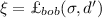; ${\xi }\in \varXi$ is the shared secret.

Initially, a trustee prepares parameters . If $P_i$ and $P_j$ wish to establish a key, they interact as follows (see Fig. 2). For simplicity, $\textsf {com}_{b, e_b}$ (resp. ver$_{b, e_b}$) for $b=1, 2$ is denoted by $\textsf {com}_{b}$ (resp. $\textsf {ver}_b$).

Fig. 2.

Our PAKE framework

• 1. $P_i$ samples $(\tau _1, y){\leftarrow } \textsf {com}_{1}(\pi _{ij})$ and sends ${y}|P_i$ to $P_j.$

• 2. Upon receiving ${y}|P_i$, $P_j$ samples $k\leftarrow D(\mathcal{K}_1)$ and derives ${U}=\alpha _1(k)$ and . Then, she derives $\varUpsilon |sk=G({\xi })$ and computes $(\tau _2, w)=\textsf {com}_{2}(\pi _{ij}; \varUpsilon )$. Next, she computes ${\omega }=w|{y}|{U}|{\sigma }|i|j$ and $\eta _0=F_{\hat{\mathcal{H}}_2(\tau _2, V)}\left( {\omega }|0\right) .$ Finally, she sends ${ w}|{U}|{\sigma }|\eta _0|P_j$ to $P_i.$

• 3. Upon receiving ${w}|{U}|{\sigma }|\eta _0|P_j$, $P_i$ computes , $\Upsilon |sk=G({\xi }),$ ${\omega }=w|{y}|{U}|{\sigma }|i|j$ and $(\tau _2, w')=\textsf {com}_{2}(\pi _{ij}; \varUpsilon )$. Then, he checks ${w}{\mathop {=}\limits ^{?}}w'$, $\eta _0{\mathop {=}\limits ^{?}}F_{\hat{\mathcal{H}}_2(\tau _2, V)}\left( {\omega }|0\right)$, $\textsf {ver}_2(\tau _2, \pi _{ij}, w){\mathop {=}\limits ^{?}}1$. If any of them fails, he rejects; otherwise, he sends $\eta _1=F_{\hat{\mathcal{H}}_2(\tau _2, V)}({\omega }|1)$ to $P_j$ and sets session key sk.

• 4. Upon receiving $\eta _1,$ $P_j$ checks $\eta _1{\mathop {=}\limits ^{?}}F_{\hat{\mathcal{H}}_2(\tau _2, V)}({\omega }|1)$. If yes, she sets session key sk; otherwise, she rejects.

3.6 Correctness

Let $\textsf {sid}_i^{\ell _i}=\textsf {sid}_j^{\ell _j}=P_i|P_j|{y}|{U}|{\sigma }$. If $P_i$ and $P_j$ share the same sid, then y is generated by $P_i$ while $({U}, {\sigma })$ is generated by $P_j$. Hence, $(\sigma , {y}, {U})$ has the specified distribution: $(\tau _1, y)\leftarrow \textsf {com}_{1}(\pi _{ij})$ and $U=\alpha _1(k)$ for $k\leftarrow D(\mathcal{K}_1)$. They will derive the same sk. Indeed, the correctness of com$_1$ implies $(\pi _{ij}, y)\in \mathcal{L}_1$. The correctness of ASPH$_B$ implies that $\textsf {Dist}[\mathcal{H}_1(k, \pi _{ij}, y), \hat{\mathcal{H}}_1(\tau , \alpha _1(k))]\le \delta$. So the correctness of implies $P_i$ and $P_j$ computes the same $\xi .$ Since $\varUpsilon |sk$ is determined by $\xi$ and the definition of PAKE correctness assumes that both $P_i$ and $P_j$ accept, they both conclude with the same sk.

3.7 Security

We now state our security theorem. The main ideas have been presented at the beginning of this section and proof details will appear in the full paper.

Theorem 1

Let be a secure one-message key reconciliation w.r.t. $(S_1, \varXi , \delta )$, $G: \varXi \rightarrow \{0, 1\}^*$ be a pseudorandom generator, and $(F, \varPhi )$ be $(1, \delta , \epsilon )$-KF MAC with key space $S_2$, domain $\mathcal{M}$ and negligible $\epsilon$. Let $\mathbb {H}_1=(\varPi _1, \textsf {ver}^*_1, \mathcal{H}_1, \hat{\mathcal{H}}_1, \alpha _1)$ be a $\delta$-ASPH$_B$ on a secure trapSim-commitment $\varPi _1=(\textsf {gen}_1, \textsf {com}_1, \textsf {ver}_1, \textsf {sim}_1)$, $\mathbb {H}_2=(\varPi _2, \textsf {ver}^*_2, \mathcal{H}_2, \hat{\mathcal{H}}_2, \alpha _2)$ be a $\delta$-${\text{ ASPH }}_A$ on a secure commitment $\varPi _2=(\textsf {gen}_2, \textsf {com}_2, \textsf {ver}_2)$. Then, our framework is secure.

4 LWE-Based Instantiation

4.1 The Learning with Errors Assumption

We next recall the Learning With Errors (LWE) assumption due to Regev [26]. For a vector $\mathbf{s}\in \mathbb {Z}_q^n$ and distribution $\chi$ over $\mathbb {Z}_q$, define distribution $A_{\mathbf{s}, \chi }$ with m samples as follows. It chooses a matrix $\mathbf{A}\leftarrow \mathbb {Z}_q^{m\times n}$, takes $\mathbf{x}\leftarrow \chi ^m$, and outputs $(\mathbf{A}, \mathbf{A}{} \mathbf{s}+\mathbf{x}).$ The decisional LWE assumption $\mathrm{DLWE}_{q, \chi , m, n}$ states that $(\mathbf{A}, \mathbf{A}{} \mathbf{s}+\mathbf{x})$ is pseudorandom when $\mathbf {s}$ is uniformly random over $\mathbb {Z}_q^n$.

For $s\in \mathbb {R}^+$, let $\varPsi _s$ be the Gaussian distribution of zero mean and standard deviation $s/\sqrt{2\pi }$. Regev [26] proved that DLWE is hard when $\chi =\varPsi _s$ with $s>2\sqrt{n}.$ Usually, it is more convenient to work with $\chi =D_{\mathbb {Z}^m, s}$. Gordon et al. [14, Lemma 2] showed that the hardness of DLWE$_{q, \Psi _s, m, n}$ implies the hardness of DLWE$_{q, D_{\mathbb {Z}^m, \sqrt{2}s}, m, n}$ when $s=\omega (\sqrt{\log n})$. For convenience, later we denote DLWE$_{q, D_{\mathbb {Z}^m, s}, m, n}$ assumption by DLWE$_{q, s, m, n}$.

4.2 Supporting Properties from LWE

  The hidden-bits lemma states that given a LWE tuple $(\mathbf{A}, \mathbf{A}{} \mathbf{s}+\mathbf{x})$, some linear function on $\mathbf{s}$ is confidential. This result is essentially a corollary of [9, Lemma C.6]. We now present it without a proof.

Lemma 9

Let $L\le n$ and $\mathbf{U}^L$ be the uniformly random variable over $\mathbb {Z}_q^L$. Let $\mathbf{C}\in \mathbb {Z}_q^{L\times (n+L)}$ be an arbitrary but fixed matrix with rank L. Then, $(\mathbf{A, As}+\mathbf{x}, \mathbf{C}{} \mathbf{s})$ and $(\mathbf{A, As}+\mathbf{x}, \mathbf{U}^{L})$ are indistinguishable under DLWE$_{q, \beta , m, n}$ assumption, where $\mathbf{A}\leftarrow \mathbb {Z}_q^{m\times (n+L)}, \mathbf{s}\leftarrow \mathbb {Z}_q^{n+L}$, $\mathbf{x}\leftarrow D_{\mathbb {Z}^m, \beta }$.

  The next lemma is adapted from [18, Lemma 3].

Lemma 10

Let $m\ge 6n\log q$ and $n\log q=o(q^{1-\alpha })$ for constant $\alpha \in (0, 1)$. Then, there is an efficient algorithm GenTrap$(1^n, 1^m, q)$ that outputs $\mathbf{A}\in \mathbb {Z}_q^{m\times n}$ and a trapdoor $\mathbf{T}\in \mathbb {Z}^{m\times m}$ such that $||\mathbf{T}||\le O(n\log q)$ and $\mathbf{A}$ is statistically close to uniform over $\mathbb {Z}_q^{m\times n}.$ Further, there exists a PPT algorithm $\textsf {BD}(\mathbf{T}, \cdot )$ that takes $\mathbf{z}\in \mathbb {Z}^m_q$ as input and does the following: if $\mathbf{z}=\mathbf{A}{} \mathbf{s}+\mathbf{x}$ with $||\mathbf{x}||_\infty \le \lfloor \frac{{q}^{\alpha }-2}{4}\rfloor$, then output $(\mathbf{t}, \mathbf{x})$; if $\mathbf{z}$ cannot be expressed in this form, then output $\perp$.

We require $m\ge 6n\log q$ (using [1, Theorem 3.2] with $||\mathbf{T}||\le O(n\log q)$), while $m\ge n\log ^2 q$ in [18] (using [1, Theorem 3.1]). However, their proof only requires $||\mathbf{T}||\cdot \frac{q^{1-\alpha }-2}{4}<q/2$. We satisfy this as $||\mathbf{T}||\le O(n\log q)=o(q^\alpha )$.

  The adaptive smoothness below states that for almost every $\mathbf{A}\in \mathbb {Z}_q^{m\times n'}$ and $\mathbf{h}\in \mathbb {Z}_q^m$, $\mathbf{E}^T(\mathbf{A}, \mathbf{v}-\mathbf{u}\odot \mathbf{h})$ are close to uniform for all but one codeword $\mathbf{u}$ in a m-length code $\mathcal{C},$ where $\mathbf{E}$ is discrete Gaussian and $\mathbf{v}$ is adaptively chosen (after given $\mathbf{E}^T\mathbf{A}$). The idea is to employ a similar result ([28, Lemma 19]) of [12, Lemma 8.3], under which we essentially only need to show that $\min _{\mathbf{s}\in \mathbb {Z}_q^{n+1}-\{\mathbf{0}\}}||(\mathbf{A}, \mathbf{v}-\mathbf{u}\odot \mathbf{h})\mathbf{s}||_\infty$ is large for all but one $\mathbf{u}\in \mathcal{C}$. Let $\mathbf{s}=(s_1, \cdots , s_{n'+1})$. Notice that Lemma 11 below implies this is true when minimizing with $s_{n'+1}\ne 0$, while case $s_{n'+1}=0$ (i.e., $\min _{\mathbf{s}'\in \mathbb {Z}_q^n-\{\mathbf{0}\}} ||\mathbf{A}{} \mathbf{s}'||_\infty$ is large for most of $\mathbf{A}$) is well known. The proof detail is given in the full paper.

Theorem 2

For $\theta \in (0, 1)$, let $s\ge {q}^{1-\frac{\theta }{3}} \cdot \omega (\sqrt{\log m})$ and $\mathcal{C}$ be a $[m, k, \theta m]_p$-code with $p<q$. Take $\mathbf{A}\leftarrow \mathbb {Z}_q^{m\times n'}, \mathbf{h}\leftarrow \mathbb {Z}_q^m$. Then, with probability $1-2^{-m}q^{n'-(1-\frac{\theta }{3}){m}}-|\mathcal{C}|^22^{-2m}q^{2n'+2-\theta m/3}$ (over $\mathbf{A}, \mathbf{h}$), the following is true for $\mathbf{E}\leftarrow (D_{\mathbb {Z}^{m}, s})^\mu$ and $\mathbf{v}=f(\mathbf{E}^T\mathbf{A})$ with an arbitrary function $f: \mathbb {Z}_q^{\mu \times n'}\rightarrow \mathbb {Z}_q^m$.

• 1. $\min _{\mathbf{s}\in \mathbb {Z}_q^{n'+1}-\{\mathbf{0}\}}||(\mathbf{A}, \mathbf{v}-\mathbf{u}\odot \mathbf{h})\mathbf{s}||_\infty \ge \lfloor \frac{q^{\theta /3}-2}{4}\rfloor$ for all but one $\mathbf{u}$ in $\mathcal{C}$;

• 2. $\mathbf{E}^T[\mathbf{A}, \mathbf{v}-\mathbf{u}\odot \mathbf{h}]$ is close to uniform in $\mathbb {Z}_q^{\mu \times (n'+1)}$ for all but the exceptional $\mathbf{u}$ in item 1.

The following lemma presents a core technique in this paper.

Lemma 11

Let $\mathbf{B}\in \mathbb {Z}_q^{m\times \nu }, \chi \in \mathbb {N}$ and $\mathbf{C}\in \mathbb {Z}_q^{m\times m}$ be arbitrary but fixed matrices with $\mathbf{C}$ invertible. Take $\mathbf{h} \leftarrow \mathbb {Z}_q^m$. Let $\mathbf{w}$ be any random variable (maybe computed from $\mathbf{h}, \mathbf{B}$) over $\mathbb {Z}_q^{m}$. Assume $\mathcal{C}$ is a $[m, k', \theta m]_p$-code for a constant $\theta \in (0, 1)$ and $p<q$. Then, with probability at least $1-|\mathcal{C}|^2q^{2\nu +2}(4\chi ^2q^{-\theta })^m$ (over choices of $\mathbf{h}$), there is at most one $\mathbf{u}\in \mathcal{C}$ that $k\mathbf{C}(\mathbf{w}-\mathbf{h}\odot \mathbf{u})=\mathbf{B}{} \mathbf{s}+\mathbf{x}$ holds for some $(k, \mathbf{s}, \mathbf{x})\in \mathbb {Z}_q^*\times \mathbb {Z}_q^\nu \times \mathbb {Z}_q^m$ with $||\mathbf{x}||_\infty < \chi$.

Proof

For any distinct $\mathbf{u}_1, \mathbf{u}_2\in \mathcal{C}$, let $\mathbf{z}_i=\mathbf{C}(\mathbf{w}-\mathbf{h}\odot \mathbf{u}_i), i=1, 2.$ Then, $\forall \mathbf{y}_1, \mathbf{y}_2\in \mathbb {Z}_q^{m}$ and $k_1, k_2\in \mathbb {Z}_q^*$, we have

$$\begin{aligned} \nonumber&P(k_1\mathbf{z}_1=k_1\mathbf{y}_1\wedge k_2\mathbf{z}_2=k_2\mathbf{y}_2) =P(\mathbf{z}_1=\mathbf{y}_1\wedge \mathbf{z}_2=\mathbf{y}_2)\\ \nonumber =&P(\mathbf{z}_1=\mathbf{y}_1\ \wedge \ (\mathbf{u}_1-\mathbf{u}_2)\odot \mathbf{h}=\varvec{\delta }), \text{ where } \varvec{\delta }=\mathbf{C}^{-1}(\mathbf{y}_1-\mathbf{y}_2)\\ \nonumber \le&P((\mathbf{u}_1-\mathbf{u}_2)\odot \mathbf{h}=\varvec{\delta })\\ \le&P(({u}_{1i}-{u}_{2i}) {h}_i=\delta _i, \forall i\in A)\quad (\text{ where } A=\{i\mid u_{1i}\ne u_{2i}, \ i\in [m]\}) \\ \nonumber \le&q^{-\theta m}\ \ (\text{ as } |A|\ge \theta m \text{ and } h_i \text{ is } \text{ uniformly } \text{ random. } ) \end{aligned}$$

(1)

Let $\mathcal{Z}\subseteq \mathbb {Z}^m$ be the cube of radius $\chi -1$ (centered at 0), and $\mathcal{S}{\mathop {=}\limits ^{def}}\cup _{\mathbf{s}\in \mathbb {Z}_q^\nu }(\mathbf{B}{} \mathbf{s}+\mathcal{Z})\cap \mathbb {Z}^{m}\mod q$. Obviously, $k\mathbf{z}=\mathbf{B}{} \mathbf{s}+\mathbf{x}$ for $||\mathbf{x}||_\infty <\chi$ is equivalent to $k\mathbf{z}\in \mathcal{S}$. Hence, $P(k_1\mathbf{z}_1\in \mathcal{S}\wedge k_2\mathbf{z}_2\in \mathcal{S})\le |\mathcal{S}|^2\cdot q^{-\theta m} =q^{2\nu }(4\chi ^2q^{-\theta })^m.$ Since $(k_1, k_2)$ has at most $q^2$ choices and $(\mathbf{u}_1, \mathbf{u}_2)$ has at most $|\mathcal{C}|^2$ choices, the bound follows. Finally, the probability bound is obtained only over choices of $\mathbf{h}$, as Eq. (1) only depends on the coins of $\mathbf{h}$ and the final result is a union bound on Eq. (1).    $\square$

Remark

The adaptiveness of $\mathbf{v}$ in Theorem 2 is important. In our PAKE, $\mathbf{E}^T\mathbf{A}$ is known to attacker. Hence, he can choose $\mathbf{v}$ based on it.

4.3 ASPHs from LWE

We will construct ASPH$_A$ and ASPH$_B$ with the following common parameters.

• n is the security parameter; prime modulus $q =n^{\lambda }$ for a constant $\lambda > \frac{3}{\theta }$ with $\theta \in (0, 1-1/\log p)$ and p a constant prime less than q; $k=o(n)$; $\delta _1=6n\log n;$ $r_1=3{n}^{1/2}$; $r_2=q^{1-\frac{\theta }{3}}{\log n}$; $\delta =q^\alpha$ (for $1-\frac{\theta }{3}+\frac{1}{\lambda }<\alpha <1$);

4.3.1 Construction of $\delta$-ASPH$_A$

Let $L\le n, \frac{7(n+L)}{\theta }\le m\le \varTheta (n)$. Take $\mathbf{g} \leftarrow \mathbb {Z}_q^{m}, \ \mathbf{B} \leftarrow \mathbb {Z}_q^{m\times (n+L)}$. Let $\mathcal{C}$ be a $[m, k, \theta m]_p$-code, constructed from Lemma 7 with negligible failure probability $mp^{(-1+\theta +1/\log p-o(1))m}$.

The Commitment Scheme. The commitment key is $(\mathbf{B}, \mathbf{g})$. To commit $\pi \in \mathbb {Z}_p^{k}$, take $\mathbf{z}\leftarrow (D_{\mathbb {Z}, r_1})^m$ and $\mathbf{t}\leftarrow \mathbb {Z}_q^{n+L}$. The commitment is $\mathbf{w}=\mathbf{B}{} \mathbf{t}+\mathbf{z}+\mathbf{g}\odot \mathcal{C}(\pi )$ with witness $\tau =(\mathbf{t}, \mathbf{z})$. The decommitment is $(\pi , \tau )$. Define $\textsf {ver}(\tau , \pi , \mathbf{w})=1$ if and only if $\mathbf{w}=\mathbf{B}{} \mathbf{t}+\mathbf{z}+\mathbf{g}\odot \mathcal{C}(\pi )$ and $||\mathbf{z}||\le \delta _1$. From $\textsf {ver}$, language $\mathcal{L}$ is generically defined. Define $\mathcal{L}^*$ so that $(\pi , \mathbf{w})\in \mathcal{L}^*$ if $||(\mathbf{B}, \mathbf{w}-\mathbf{g}\odot \mathcal{C}(\pi ))\mathbf{s}||_\infty <\lfloor \frac{q^{\theta /3}-2}{4}\rfloor$ for some $\mathbf{s}\in \mathbb {Z}_q^{n+L+1}-\{\mathbf{0}\}$.

Lemma 12

Our commitment is secure under DLWE$_{q, r_1, m, n}$ assumption.

Proof

Consider correctness first. Let $\mathbf{w}=\mathbf{B}{} \mathbf{t}+\mathbf{g}\odot \mathcal{C}(\pi )+\mathbf{z}$ be a commitment of $\pi$ with $\mathbf{z}\leftarrow D_{\mathbb {Z}^m, r_1}$. Then, correctness holds if $||\mathbf{z}||\le \delta _1$, which is true except for probability $O(2^{-m})$, by Lemma 2 (noticing $r_1\sqrt{m}=\varTheta (n)=o(\delta _1)$). Hiding property directly follows from DLWE$_{q, r_1, m, n}$ assumption. The binding property follows from the properties of $\mathcal{L}^*$ (to be verified soon): $\mathcal{L}\subseteq \mathcal{L}^*$ and for any $\mathbf{w}\in \mathbb {Z}_q^m$, there is only one $\pi$ so that $(\pi , \mathbf{w})\in \mathcal{L}^*.$    $\square$

Description of $\delta$-ASPH$_A$. We verify the required properties for $\mathcal{L}^*$.

• 1. $\mathcal{L}\subseteq \mathcal{L}^*.$ This is obvious as $||\cdot ||_\infty \le ||\cdot ||$ and $\delta _1=o(q^{\theta /3})$ using $\lambda \theta /3>1$.

• 2. For any $\mathbf{w}\in \mathbb {Z}_q^m$,there is at most one $\pi \in \mathbb {Z}_p^k$ with $(\pi , \mathbf{w})\in \mathcal{L}^*$. This directly follows from Theorem 2(1) (with $n'=n+L$), where the exception probability is $O(q^{(-1/3+o(1))n})$ (negligible!).

We define $\mathcal{H}$ and $\hat{\mathcal{H}}$. For secret $\mathbf{O}\leftarrow (D_{\mathbb {Z}, r_2})^{m\times L}$, let the projection key $\mathbf{V}=\mathbf{O}^T\mathbf{B}$. Let $\mathcal{H}(\mathbf{O}, \pi , \mathbf{w})=\mathbf{O}^T(\mathbf{w}-\mathbf{g}\odot \mathcal{C}(\pi )).$ If $(\pi , \mathbf{w})\in \mathcal{L}$ with witness $\tau =(\mathbf{t}, \mathbf{z})$, let $\hat{\mathcal{H}}(\tau , \mathbf{V})=\mathbf{V}{} \mathbf{t}$.

Correctness. Assume the closeness uses the $||\cdot ||_\infty$ metric. Let $(\pi , \mathbf{w})\in \mathcal{L}$. Then, $\mathbf{w}=\mathbf{B}{} \mathbf{t}+\mathbf{g}\odot \mathcal{C}(\pi )+\mathbf{z}$ with $||\mathbf{z}||\le \delta _1$. For $\mathbf{O}\leftarrow (D_{\mathbb {Z}, r_2})^{m\times L}$, we have $||\mathbf{V}{} \mathbf{t}-\mathbf{O}^T(\mathbf{w}-\mathbf{g}\odot \mathcal{C}(\pi ))||_\infty =\max _i|\mathbf{o}_i^T\mathbf{z}|\le \delta _1 r_2\log n=o(\delta )$ (except for a negligible probability by Lemma 2), where $\mathbf{o}_i$ is the ith column of $\mathbf{O}.$

Adaptive Smoothness. For $(\pi , \mathbf{w})\not \in \mathcal{L}^*$, $\mathcal{C}(\pi )$ is not the exceptional $\mathbf{u}$ in Theorem 2 and hence $\mathbf{O}^T(\mathbf{B}, \mathbf{w}-\mathbf{g}\odot \mathcal{C}(\pi ))$ is close to uniform over $\mathbb {Z}_q^{L\times (n+L+1)}.$ Further, under our setup ($n'=n+L, m\ge \frac{7(n+L)}{\theta }, k=o(n)$), the exceptional probability for Theorem 2 is $O(q^{-(1/3+o(1))n})$ (negligible).

Strong Smoothness. We need to show that $(\mathbf{O}^T\mathbf{B}, \mathbf{B}{} \mathbf{t}+\mathbf{z}, \mathbf{O}^T\mathbf{B}{} \mathbf{t})$ is indistinguishable from $(\mathbf{O}^T\mathbf{B}, \mathbf{B}{} \mathbf{t}+\mathbf{z}, \mathbf{U})$, where $(\mathbf{z}, \mathbf{t}, \mathbf{O}, \mathbf{U})\leftarrow (D_{\mathbb {Z}, r_1})^{m}\times \mathbb {Z}_q^{n+L}\times (D_{\mathbb {Z}, r_2})^{m\times L}\times \mathbb {Z}_q^{L}$. This follows from Lemma 9, as $\mathbf{O}^T\mathbf{B}$ is close to uniform (well-known and also implied by Theorem 2) and hence has a rank $<L$ only negligibly.

4.3.2 Construction of $\delta$-ASPH$_B$

$\delta$-ASPH$_B$ is identical to $\delta$-ASPH$_A$, except that we need a trapdoor property while strong smoothness is no longer needed. Even though, we still need to validate claims adapted from $\delta$-ASPH$_A$ under our new parameter choices. This is shown below in the security item. The trapdoor property is from Lemma 10.

Let $\mu \in \mathbb {N}, m=6n\log n$. Take $\mathbf{h}\leftarrow \mathbb {Z}_q^m, \mathbf{A} \leftarrow \mathbb {Z}_q^{m\times n}$. $\mathcal{C}$ is a $[m, k, \theta m]_p$-code (from Lemma 7 with a negligible failure probability $mp^{(-1+\theta +1/\log p-o(1))m}$).

trapSim-commitment Scheme. The commitment key is $(\mathbf{A}, \mathbf{h})$. The commitment to $\pi \in \mathbb {Z}_p^{k}$ is $\mathbf{y}=\mathbf{A}{} \mathbf{s}+\mathbf{x}+\mathbf{h}\odot \mathcal{C}(\pi )$ for $\mathbf{x}\leftarrow (D_{\mathbb {Z}, r_1})^m$ and $\mathbf{s}\leftarrow \mathbb {Z}_q^m$ with witness $\tau =(\mathbf{s}, \mathbf{x})$. Further, $\textsf {ver}, \mathcal{L},$ and $\mathcal{L}^*$ are defined the same as in $\delta$-ASPH$_A$ via equation $\mathbf{y}=\mathbf{A}{} \mathbf{s}+\mathbf{x}+\mathbf{h}\odot \mathcal{C}(\pi )$. The trapdoor simulation is to apply Lemma 10 to generate $\mathbf{A}$ with trapdoor $\mathbf{T}\in \mathbb {Z}^{m\times m}$, by setting $\alpha =\theta /3$ and noticing that $n\log q=o(q^{1-\theta /3})$ (as $\lambda (1-\theta /3)\ge 2\lambda /3\ge 2$, due to $\lambda >\frac{3}{\theta }\ge 3$).

For $(\mathbf{A}, \textsf {T})\leftarrow \textsf {TrapGen}(1^n)$, membership $(\pi , \mathbf{y})\in \mathcal{L}^*$ can be verified as follows. For each $u\in \mathbb {Z}_q^*$, try to use T to recover $(\mathbf{s}, \mathbf{x})$ so that $u(\mathbf{y}-\mathbf{h}\odot \mathcal{C}(\pi ))=\mathbf{A}{} \mathbf{s}+\mathbf{x}$ with $||\mathbf{x}||_\infty \le \lfloor \frac{q^{\theta /3}-2}{4}\rfloor$. If it succeeds for some u, then claim $(\pi , \mathbf{y})\in \mathcal{L}^*$; otherwise, claim $(m, \mathbf{y})\not \in \mathcal{L}^*.$ By Lemma 10, this decision is always correct.

Description of $\delta$-ASPH$_B$. This is identical to $\delta$-ASPH$_A$. For secret $\mathbf{E}\leftarrow D_{\mathbb {Z}, r_2}^{m\times \mu }$, the projection key is $\mathbf{U}=\mathbf{E}^T\mathbf{A}$. Also, let $\mathcal{H}(\mathbf{E}, \pi , \mathbf{y})=\mathbf{E}^T(\mathbf{y}-\mathbf{h}\odot \mathcal{C}(\pi )).$ If $(\pi , \mathbf{y})\in \mathcal{L}$ with witness $\tau =(\mathbf{s}, \mathbf{x})$, let $\hat{\mathcal{H}}(\tau , \mathbf{U})=\mathbf{U}{} \mathbf{s}$.

Security. Security proofs for commitment, correctness and adaptive smoothness are identical to $\delta$-ASPH$_A$. However, we need to verify that the cited results have negligible exception probabilities under our setup. Commitment security has used Lemma 2 to correctness. In our setting, $r_1\sqrt{m}=\varTheta (n\sqrt{\log n})=o(\delta _1)$ still holds and so the result remains valid. The correctness has cited Lemma 2 which requires $\delta _1r_1\log n=o(\delta )$ and remains valid in our setting. Theorem 2 is cited for smoothness and property 2 of $\mathcal{L}^*$. In our setting, it only has negligible exception probability $O(q^{(-\theta /3+o(1))m})$.

4.4 LWE-Based PAKE Instantiation

Using $\delta$-ASPH$_B$ and $\delta$-${\text{ ASPH }}_A$ just obtained, together with pseudorandom generator G, KF-MAC F (in Sect. 3.3) and reconciliation (in Sect. 3.2), we can realize our PAKE framework in the LWE setting (see Fig. 3). By the security theorem of PAKE framework, we only need to make sure that each of these mechanisms is secure in our parameter choices. This is specified as follow.

• $\theta \in (0, 1-1/\log p)$; $q=n^\lambda$ ($\lambda >\frac{3}{\theta }$); p is constant prime with $p<q$; $k=o(n)$; $r_1= 3{n}^{\frac{1}{2}}$, $\delta _1=6n\log n,$ $r_2=q^{1-\frac{\theta }{3}}{\log n}$, $\delta =q^\alpha$ with $1-\frac{\theta }{3}+\frac{1}{\lambda }<\alpha <1$.

• $G: \{0, 1\}^{L'}\rightarrow \{0, 1\}^*$ is a pseudorandom generator.

• password dictionary $\mathcal{D}\subsetneq \mathbb {Z}_p^{k}$.

• Instantiate KF-MAC. Set $F_K$ as the $(1, \delta , (\frac{4\delta }{q})^{\theta _{mac} L/p})$-KF MAC in Sect. 3.3 with key space $\mathbb {Z}_q^{L}$, where $\theta _{mac}\in (0, 1-1/\log p)$, $L=\frac{k_2p(1+\beta )}{1-\theta _{mac}-1/\log p}$ for constant $\beta >0$ (where $k_2=o(n)$ is the p-ary output length of H in $F_K$). /* In this setup, insecurity error $(\frac{4\delta }{q})^{\theta _{mac} L/p}=(4q^{\alpha -1})^{\varTheta (k_2)}$ (negligible); $[L/p, k_2, \theta _{mac}L/p]_p$-code in the scheme is constructed from Lemma 7 with negligible exception probability $O(p^{-k_2\beta }L/p)$. */

• Instantiate $(\mathcal{H}_1, \hat{\mathcal{H}}_1)$ with our LWE-based $\delta$-ASPH$_B$: Set $m=6n\log n$, $\mu =L'\log \frac{q}{16\delta }$ ($L'$ is the key length of G); other parameters such as $\delta _1, \delta , r_2, r_1$ are set as above; $[m, k, \theta m]_p$-code $\mathcal{C}$ is from Lemma 7. Take $\mathbf{A}\leftarrow \mathbb {Z}_q^{m\times n}, \mathbf{h}\leftarrow \mathbb {Z}_q^m$. /* Under our setup, $\mathcal{C}$ fails to be constructed by Lemma 7 only with negligible probability $m p^{(-1+\theta +1/\log p)m}$; our setup is consistent with parameter description in $\delta$-ASPH$_B$ and hence the resulting scheme is secure. */

• Instantiate $(\mathcal{H}_2, \hat{\mathcal{H}}_2)$ with our LWE-based $\delta$-ASPH$_A$: Set $m_1= \frac{7(L+n)}{\theta }$; $\delta _1, \delta , r_2, r_1, L$ etc set as above; $[m_1, k, \theta m_1]_p$-code $\mathcal{C}_1$ is from Lemma 7. Take $\mathbf{B}\leftarrow \mathbb {Z}_q^{m_1\times (n+L)}$ and $\mathbf{g}\leftarrow \mathbb {Z}_q^{m_1}$ as public parameters for $\delta$-ASPH$_A$. /* Under our setup, $\mathcal{C}_1$ fails to be constructed by Lemma 7 only with negligible probability $m_1p^{(-1+\theta +1/\log p)m_1}$; our setup is consistent with parameter description in $\delta$-ASPH$_A$ and hence the resulting scheme is secure. */

• Set $\mathbf{V}=\mathbf{O}^T\mathbf{B} \in \mathbb {Z}_q^{L \times (n+L)}$ for $\mathbf{O}\leftarrow (D_{\mathbb {Z}^{m_1}, r_2})^{L}$ as the public projection key.

• For ${\pi }\in \mathbb {Z}_p^k$, define $\mathbf{g}_\pi =\mathbf{g}\odot \mathcal{C}_1(\pi )$ and $\mathbf{h}_\pi =\mathbf{h}\odot \mathcal{C}(\pi )$.

• Instantiate . Set as the reconciliation scheme in Sect. 3.2 with $\mu , \delta$ and q as above. Thus, the reconciliated key $\varvec{\xi }$ has a bit-length at least $\mu \log \frac{q}{16\delta }=L'$ (fit the key length of G).

The public parameter list for our PAKE is . The detailed protocol is simply to plug the primitives above into our PAKE framework. This is graphically shown in Fig. 3. Since primitives are secure by our parameter clarification, our protocol is secure by Theorem 1.

Fig. 3.

Our Protocol LWE-PAKE: $\mathbf{t}\leftarrow \mathbb {Z}_q^{n+L}$ and $\mathbf{z}\leftarrow D_{\mathbb {Z}^{m_1}, r_1}$ are sampled with randomness $\varUpsilon$ where $\varUpsilon |sk=G(\varvec{\xi })$.

Efficiency. Note that $\mathbf{g}_{\pi _{ij}}$ and $\mathbf{h}_{\pi _{ij}}$ can be pre-computed and $D_{\mathbb {Z}, r}^m$ can be sampled in $\tilde{O}(m)$ time [23]. Thus, the cost of $P_i$ is dominated by $\mathbf{B}{} \mathbf{t}, \mathbf{Us}, \mathbf{A}{} \mathbf{s}$ and $\mathbf{V}{} \mathbf{t}$ which totally is about mn multiplications over $\mathbb {Z}_q$ (as $L= O(n), \mu =O(n)$ and $m_1=o(m)$); the cost of $\mathbf{P}_j$ is dominated by $\mathbf{E}^T\mathbf{A}, \mathbf{E}^T\mathbf{y}', \mathbf{Bt}, \mathbf{Vt}$ which is $\mu mn =O(L'mn/\log q)$ multiplications. The communication cost is dominated by $(\mathbf{U}, \mathbf{w}, \mathbf{y})$ which has $O(\frac{L'n}{\log n}+n\log n)$ field elements. Finally, the authentication is provided by $(\mathbf{w}, \eta _0)$ with a cost dominated by $\mathbf{Bt}$ and $\mathbf{Vt}$, which is $(m_1+L)(n+L)=O(n^2)$ multiplications. This is more efficient than authentication [6, 15] from CCA-secure encryption, which has a cost $O(n^2\log n)$ [21, 29] in the LWE setting. Our main saving for this comes from the fact that $\delta$-ASPH$_A$ doesn’t need a trapdoor simulation so it can take $m_1=O(n)$ while [21, 29] needs this and hence the corresponding parameter is $O(n\log n)$. That is, authentication data $(w, \eta _0)$ can not enable to decrypt $\pi _{ij}$ and so it is different from authentication by CCA-secure encryption.

5 Instantiation from Ring-LWE

This section will present our PAKE instantiation based on Ring-LWE. This is important as it is more efficient than LWE-based one.

5.1 Basics of Rings, Ring-LWE and Operational Properties

5.1.1 Introduction to Algebraic Number Theory

We provide some facts from algebraic number theory (also see [20]). Let m be a power of 2 and $n=m/2.$

Power Basis of Cyclotomic Field. We are interested in the mth cyclotomic field $K=\mathbb {Q}(\zeta _m)$, where $\zeta _m$ is the mth primitive root of unity and has the minimal polynomial $\varPhi _m(x)=x^n+1$ with $n=m/2$. Then, K has a $\mathbb {Q}$-basis $\{1, \zeta _m, \zeta _m^2, \cdots , \zeta _m^{n-1}\}$ (called power basis, denoted by $\mathbf{p}$).

Canonical Embedding. $K=\mathbb {Q}(\zeta _m)$ has n embeddings $\sigma _i: K\rightarrow \mathbb {C}$, $\forall i\in \mathbb {Z}_m^*$. The canonical embedding $\sigma : K\rightarrow \mathbb {C}^{\phi (m)}$ is $\sigma (a)=(\sigma _i(a))_{i\in \mathbb {Z}_m^*}$ for $a\in K$. Since $\sigma _i(a)=\bar{\sigma }_{m-i}(a)$, $\sigma (a)\in H.$

Ring of Integers and Ideals. An algebraic integer in K is an element in it that is a root of a monic polynomial in $\mathbb {Z}[x].$ The set of all integers of K is a ring, denoted by R in this paper. For $K=\mathbb {Q}(\zeta _m)$, $R=\mathbb {Z}[\zeta _m].$ Thus, the power basis $\{1, \zeta _m, \cdots , \zeta _m^{n-1}\}$ is a $\mathbb {Z}$-basis of R.

Chinese Remainder Basis and Its Relation with Power Basis. In this paper, q is a prime with $q=1\mod m$ and $\omega _m$ is the mth root of 1 in $\mathbb {Z}_q^*.$ let $\mathfrak {p}_i=(q, \zeta _m-\omega _m^i)$ (i.e., the ring generated by q and $\zeta _m-\omega _m^i).$ By Chinese remainder theorem, for each $i\in \mathbb {Z}_m^*$, there exists $c_i\in R$ so that $c_i=1\mod \mathfrak {p}_i$ and $c_i=0\mod \mathfrak {p}_j$ for any $j\ne i.$ Then, $\mathbf{c}=(c_j)_{j\in \mathbb {Z}_m^*}$ forms a basis of $R_q{\mathop {=}\limits ^{def}}R \text{ mod } q,$ called the CRT basis. Note that $c_i^2=c_i \mod qR$, as $c_i^2=c_i\mod \mathfrak {p}_i$ for each $i\in \mathbb {Z}_m^*.$ Hence, if $a=\mathbf{c}^T\mathbf{v}, b=\mathbf{c}^T\mathbf{u}\in R_q$ for $\mathbf{v}, \mathbf{u}\in \mathbb {Z}_q^{n}$, then $ab=\mathbf{c}^T(\mathbf{v}\odot \mathbf{u})$. Let $\text{ CRT }_m=(\omega _m^{ij})_{i\in \mathbb {Z}_m^*, j\in [n]}.$ Then, the power basis p and CRT basis c is connected by $\mathbf{p}^T=\mathbf{c}^T\cdot \text{ CRT }_m$. Thus, if $a=\mathbf{p}^T\mathbf{v}$ for some $\mathbf{v}\in \mathbb {Z}_q^{n},$ then $a=\mathbf{c}^T\cdot \text{ CRT }_m\mathbf{v}$.

Coefficient Vector Representation. For $a=\mathbf{p}^T\mathbf{v}$ with some $\mathbf{v}\in \mathbb {Z}_q^n,$ we call $\mathbf{v}$ the coefficient vector of a under $\mathbf{p}$ and denote it by $\underline{a}.$ For $\mathbf{a}\in R_q^\ell$, let $\mathbf{a}=(\mathbf{p}^T\mathbf{v}_1,\cdots , \mathbf{p}^T\mathbf{v}_\ell )^T$ for some $\mathbf{v}_i\in \mathbb {Z}_q^n$. We call $(\mathbf{v}_1; \cdots ; \mathbf{v}_\ell )$ the coefficient vector of $\mathbf{a}$ under $\mathbf{p}$ and denote it by $\underline{\mathbf{a}}$. Similarly, we can define the coefficient vector of a and $\mathbf{a}$ under basis $\mathbf{c}$ and denote them by and respectively. As $\mathbf{p}^T=\mathbf{c}^T\cdot \text{ CRT }_m$, we know that For $\mathbf{a}\in R_q^{\ell }$, we have and

5.1.2 Gaussian Samplings

Gaussian Distribution over $K\otimes \mathbb {R}$. Since m is a power of 2, the power basis $\mathbf{p}$ is an orthogonal basis of H (via canonical embedding $\sigma$ and [20, Lemma 2.15]) and $||\zeta _m^j||=\sqrt{n}$, $\forall j\in \mathbb {Z}_m^*$. Hence, Gaussian distribution over $K\otimes \mathbb {R}$ (or H via $\sigma$) with parameter $\xi$ can be sampled as $\mathbf{z}=\sum _{i=0}^{n-1}\zeta _m^jr_j$, where $r_0, \cdots , r_{n-1}$ is i.i.d. Gaussian over $\mathbb {R}$ with parameter $\xi /\sqrt{n}$. Denote this distribution by $\varPsi _\xi$.

Discrete Gaussian over R. Since $\mathbf{p}$ is an orthogonal basis of R (embedded into H), $\mathbf{e}=\sum _{i=0}^{n-1} \zeta _m^j e_i$ with $e_i\leftarrow D_{\mathbb {Z}, s/\sqrt{n}}$ is according to $D_{R, s}$.

5.1.3 Ring-LWE

The Learning With Errors over rings (Ring-LWE) was introduced in [19], where the worst-case hardness result was also proven. Based on basis $\mathbf{p}$, $x\in K\otimes \mathbb {R}$ can be represented as $x=\sum _i x_i\zeta _m^i$ for $x_i\in \mathbb {R}.$ Also, $x\in K/qR\otimes \mathbb {R}$ can be represented as $x=\sum _i x_i\zeta _m^i$ for $x_i\in [0, q).$ Let $\mathbb {T}=K/qR\otimes \mathbb {R}.$

For $s\in R_q$ and distribution $\chi$ over $K\otimes \mathbb {R},$ a sample from distribution $A_{s, \chi }$ over $R_q\times \mathbb {T}$ consists of (a, b) with $a\leftarrow R_q, e\leftarrow \chi$ and $b=as+e \mod q.$

Decisional ring-LWE (ring-DLWE$_{q, \chi , m}$) states that independent samples from $A_{s, \chi }$ for $s\leftarrow R_q$ and the same number of samples uniformly over $R_q\times \mathbb {T}$ are indistinguishable. Denote this assumption with $\chi =D_{R, r}$ by ring-DLWE$_{q, r, m}$.

5.1.4 Matrix Representations for Operations over $R_q$

In this subsection, we will give some useful facts on the matrix representation over $\mathbb {Z}_q$ for elements, vector or matrix over $R_q$. For $b\in R_q$, define , . Generally, for $\mathbf{D}=(d_{ij})\in R_q^{\ell \times k}$ and $u=1, 2$, define $\phi _u(\mathbf{D})=(\phi _u(d_{ij}))_{1\le i\le \ell , 1\le j\le k}$ (a block matrix with entry (i, j) being $\phi _u(d_{ij})$). For $\mathbf{v}\in \mathbb {Z}_q^n$, define $\ddag (\mathbf{v})=\left[ \begin{array}{cccc} v_0&{} v_{1} &{} \cdots &{} v_{n-1}\\ -v_{n-1}&{} v_0&{} \cdots &{} v_{n-2}\\ \vdots &{} \vdots &{} \ddots &{} \vdots \\ -v_{1} &{} -v_{2} &{} \cdots &{} v_{0}\end{array} \right]$. The following facts about $\phi _1, \phi _2, \ddag$ are useful.

Lemma 13

Let $s\in R_q, \mathbf{e}, \mathbf{b}\in R_q^\ell$ and $\mathbf{D}=(\mathbf{d}^{(1)}, \cdots , \mathbf{d}^{(k)})\in R_q^{\ell \times k}$.

• 1.
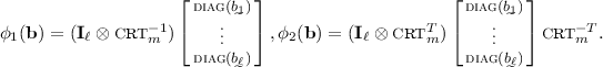
• 2.

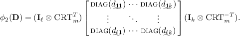
• 3. .

• 4. $[\underline{\mathbf{e}^T\mathbf{b}}]^T=[\underline{\mathbf{e}}]^T\phi _2(\mathbf{b})$. Further, $((\underline{\mathbf{e}^T \mathbf{d}^{(1)}})^T, \cdots , (\underline{\mathbf{e}^T\mathbf{d}^{(k)}})^T)= [\underline{\mathbf{e}}]^T \cdot \phi _2(\mathbf{D}).$

• 5. $\phi _2(s)=\ddag (\underline{s}).$

Proof

Items 1 and 2 follow by definition. For item 3, notice that for $s, b\in R_q$, Generalizing to $\mathbf{b}\in R_q^{\ell }$ follows by definition of $\phi _1(\mathbf{b}).$ For item 4, notice for $s, b\in R_q$. Thus, $[\underline{\mathbf{e}^T\mathbf{b}}]^T=\sum _i [\underline{e_ib_i}]^T=\sum _i [\underline{e}_i]^T\phi _2(b_i)=[\underline{\mathbf{e}}]^T\phi _2(\mathbf{b}).$ Generalizing to the second part of item 4 follows by definition of $\phi _2(\mathbf{D}).$ For item 5, notice that $[\underline{bs}]^T=\underline{s}^T\cdot \ddag (\underline{b})$ (as $x^n+1=0$ in $R_q$). But we know that $[\underline{bs}]^T=\underline{s}^T\cdot \phi _2(b)$. Since s is arbitrary in $R_q$, the result follows.    $\square$

In the remaining of this section, we will present materials for ring-LWE based PAKE instantiation. Due to the space limitation, we present it in the intuitive level. The formal details appear in the full paper.

5.2 Supporting Properties from Ring-LWE

Regularity. We prove a regularity result: for discrete Gaussian $\mathbf{e}$ over $R^{\ell }$ and uniformly random $\mathbf{D}$ over $R_q^{\ell \times k}$, $\mathbf{e}^T\mathbf{D}$ is statistically close to uniform over $R_q^{k}$ (for quite general $k, \ell$). The strategy is as follows. By Lemma 13(4), ${\mathbf{e}^T\mathbf{D}}$ is represented by $[\underline{\mathbf{e}}]^T\phi _2(\mathbf{D})$. It suffices to show that $[\underline{\mathbf{e}}]^T\phi _2(\mathbf{D})$ is close to uniform in $\mathbb {Z}_q^{1\times nk}$. We use Lemma 3 (with Lemma 1) to do this. This essentially only requires to show that $\min _{\mathbf{s}\in \mathbb {Z}_q^{kn}-\{\mathbf{0}\}}||{ \phi _2(\mathbf{D})}{} \mathbf{s}||_\infty$ is large, as it implies a full column rank of $\phi _2(\mathbf{D})$ and large $\lambda _1^\infty (\varLambda (\phi _2(\mathbf{D})))$. This requirement is shown in the full paper. It should be noted that our regularity result with a special form of $\mathbf{D}$ appeared in [20] while the case of $k=1$ is in [10].

Adaptive Smoothness-I. Given $\mathbf{a}, \mathbf{h}\leftarrow R_q^{\ell }$ and a $[\ell n, k, d]_p$-code $\mathcal{C}$ with large d, we show the following holds with high probability (over $\mathbf{a}, \mathbf{h}$): let $\mathbf{E}$ be discrete Gaussian over $\mathbb {Z}^{\ell n\times \mu }$ and $\mathbf{w}$ be adaptively chosen after given $\mathbf{E}^T\cdot \phi _1(\mathbf{a}).$ Then,

• 1. $\min _{\mathbf{s}\in \mathbb {Z}_q^{n+1}-\mathbf{0}}||\Big (\phi _1(\mathbf{a}), \underline{\mathbf{w}-\mathbf{h}_\mathbf{u}}\Big )\mathbf{s}||_\infty$ is large for all but one $\mathbf{u}$ in $\mathcal{C}$, where $\mathbf{h}_\mathbf{u} \in R_q^\ell$ is defined so that ;

• 2. $\mathbf{E}^T\Big (\phi _1(\mathbf{a}), \underline{\mathbf{w}-\mathbf{h}_\mathbf{u}}\Big )$ is close to uniform over $\mathbb {Z}_q^{\mu \times (n+1)}$ for all $\mathbf{u}\in \mathcal{C}$ but the exceptional one in item 1, where the statistical closeness is over $\mathbf{E}.$

To show item 1, it suffices to show $||\phi _1(\mathbf{a})\cdot \mathbf{s}'||_\infty$ for any $\mathbf{s}'\in \mathbb {Z}_q^n-\{\mathbf{0}\}$ is large and the $||\cdot ||_\infty$-distance from $t(\underline{\mathbf{w}-\mathbf{h}_\mathbf{u}})$ to $\mathcal{L}(\phi _1(\mathbf{a}))$, $\forall t\in \mathbb {Z}_q^*$, is large for all but one $\mathbf{u}$ in $\mathcal{C}$. The former is given by a random argument and the latter is a consequence of Lemma 11, using . Item 2 follows from the adaptive version of Lemma 3, using item 1.

Adaptive Smoothness-II. In smoothness-I, we can extract $\mu$ random elements in $\mathbb {Z}_q$ (i.e., $\mathbf{E}^T(\underline{\mathbf{w}-\mathbf{h}_\mathbf{u}})$) from $\mu \times n$ matrix $\mathbf{E}^T\phi _1(\mathbf{a})$. In smoothness-II, we show this extraction efficiency can be improved. Specifically, for $\mathbf{D}\leftarrow R_q^{\ell \times k}, \mathbf{h}\leftarrow R_q^\ell$ and a $[\ell n, k', d]_p$-code $\mathcal{C}$ with large d, we show the following holds with high probability (over $\mathbf{D}, \mathbf{h}$). Let $\mathbf{e}$ be discrete Gaussian in $R^\ell$ and $\mathbf{w}$ is adaptively chosen after given $\mathbf{e}^T\mathbf{D}.$

• 1. $\min _{\mathbf{s}\in \mathbb {Z}_q^{kn+L}-\mathbf{0}}||\Big (\phi _2(\mathbf{D}), \phi _2(\mathbf{w}-\mathbf{h}_\mathbf{u})_L\Big )\mathbf{s}||_\infty$ is large for all but one $\mathbf{u}$ in $\mathcal{C}$, where $\mathbf{h}_\mathbf{u} \in R_q^\ell$ is defined s.t. and $\phi _2(\mathbf{v})_L$ is the first L columns of $\phi _2(\mathbf{v}).$

• 2. $(\mathbf{e}^T\mathbf{D}, [\underline{\mathbf{e}^T(\mathbf{w}-\mathbf{h}_\mathbf{u})}]_1^L)$ is close to uniform in $R_q^k\times \mathbb {Z}_q^L$ for all $\mathbf{u}\in \mathcal{C}$ but the exceptional one in item 1, where $[\mathbf{x}]_1^L$ is the first L components of vector $\mathbf{x}$ and the statistical closeness is over $\mathbf{e}.$

Here $k\in \mathbb {N}$ is arbitrary (e.g. $k=1$ and later we will take $k=2$). The parameter $L<n$ but we can achieve $L=\varTheta (n).$ Consequently, we can now extract $\varTheta (n)$ elements in $\mathbb {Z}_q$ from $\mathbf{e}^T\mathbf{D}\in R^k_q$. The proof of item 1 is given by a strengthened regularity. The idea of item 2 is to use Lemma 13(4) to study the distribution of its matrix form $[\underline{\mathbf{e}}]^T(\phi _2(\mathbf{D}), \phi _2(\mathbf{w}-\mathbf{h}_u)_L)$. This is provably close to uniform for all but one $\mathbf{u}$ by item 1 and a variant of [28, Lemma 19].

Hidden-Bits Lemma from Ring-LWE. We extend LWE-based hidden-bits lemma in Sect. 4.2 to the ring-LWE setting. It essentially says that given a redundant ring-LWE tuple, we can extract some random bits of the secret that is confidential to an attacker. Formally, for fixed $\alpha , \beta \in R_q$, let Then, given $\mathbf{a}, \mathbf{b}\leftarrow {R}_q^{\ell }$ and $\mathbf{a}s+\mathbf{b}t+\mathbf{x}$ for $s, {t}\leftarrow R_q$ and $\mathbf{x}$ discrete Gaussian over $R^\ell$, it holds that $\left[ \ \underline{\alpha {s}+\beta {t}}\ \right] _1^L$ is indistinguishable from uniformly random in $\mathbb {Z}_q^L$ under the ring-DLWE assumption.

Trapdoor Generation from Ring-LWE. We generalize the trapdoor generation algorithm in $\mathbb {Z}^m$ in [21] to the ring-LWE setting. The algorithm will generate a random matrix $\mathbf{D}\in R_q^{\ell \times \nu }$ together with a trapdoor $\mathbf{R}$ so that $\mathbf{R}$ can be used to decode $\mathbf{t}$ from $\mathbf{D}{} \mathbf{t}+\mathbf{x}$ when $\underline{\mathbf{x}}$ is short. Ducas and Micciancio [10] obtained the generalization for case $\nu =1$. We obtain the result for the general $\nu$ case. Our algorithm is simply the ring version of [21]: $\mathbf{D}=(\mathbf{D}_0; \mathbf{I}_\nu \otimes \mathbf{g}-\mathbf{R}^T\mathbf{D}_0)$ for a random matrix $\mathbf{D}_0$ in $R_q^{(\ell -k\nu )\times \nu }$ and a discrete Gaussian matrix $\mathbf{R}$ in $R^{(\ell -k\nu )\times k\nu }$, where $\mathbf{g}=(1, 2, \cdots , 2^{k-1})^T$ and $k=\lceil \log q\rceil$. To show that $\mathbf{D}$ is random, it requires to show that given $\mathbf{D}_0$, $\mathbf{R}^T\mathbf{D}_0$ is statistically random. This follows by our regularity result above. The decoding property is a trivial extension of [21].

5.3 ASPHs from Ideal Lattices

In this section, we will present our construction of ASPH from ideal lattices. The idea is to extend the LWE-based schemes to the ring-LWE setting.

5.3.1 Construction of $\delta$-${\text {ASPH}}_A$

Let $L\le n, \theta \in (0, 1), k=o(n), \ell \in \mathbb {N}, p$ constant prime. Take $\mathbf{g} \leftarrow R_q^{\ell }, \ \mathbf{D}=(\mathbf{d}_1, \mathbf{d}_2) \leftarrow R_q^{\ell \times 2}$. Let $\mathcal{C}$ be a $[\ell n, k, \theta \ell n]_p$-code. For $\pi \in \mathbb {Z}_p^k$, define $\mathbf{g}_\pi \in R_q^\ell$ such that

The Commitment Scheme. The commitment key is $(\mathbf{D}, \mathbf{g})$. To commit to $\pi \in \mathbb {Z}_p^k$, take $\mathbf{t}\leftarrow R_q^{2}$ and $\mathbf{z}$ discrete Gaussian over $R^\ell$. The commitment is $\mathbf{w}=\mathbf{D}{} \mathbf{t}+\mathbf{g}_{\pi }+\mathbf{z}$ with witness $(\mathbf{t}, \mathbf{z})$. The decommitment is $({\pi }, \mathbf{t}, \mathbf{z})$. Let $\textsf {ver}(\mathbf{t}, \mathbf{z}, {\pi }, \mathbf{w})=1$ if and only if $\mathbf{w}=\mathbf{D}{} \mathbf{t}+\mathbf{g}_{\pi }+\mathbf{z}$ with $||\underline{\mathbf{z}}||$ small.

Then, we define $\mathcal{L}$ and $\mathcal{L}^*$. Let $\mathcal{X}=\mathbb {Z}_p^k\times R_q^{\ell }$. Then, $\mathcal{L}$ is generically defined by $\textsf {ver}.$ Define $\mathcal{L}^*=\{({\pi }, \mathbf{w})\in \mathcal{X}\mid ||\Big (\phi _2(\mathbf{D}), \phi _2(\mathbf{w}-\mathbf{g}_\pi )_L\Big )\mathbf{s}||_\infty \text{ is } \text{ small } \text{ for } \text{ some } \mathbf{s}\in \mathbb {Z}_q^{2n+L}-\{\mathbf{0}\} \}$, where $\phi _2(\mathbf{v})_L$ is the first L columns of matrix $\phi _2(\mathbf{v}).$

Our commitment is secure: the hiding property directly follows from ring-DLWE assumption and binding property is implied by properties of $\mathcal{L}^*$:

(1) $\mathcal{L}\subseteq \mathcal{L}^*$. This is true as $||\Big (\phi _2(\mathbf{D}), \phi _2(\mathbf{D}{} \mathbf{t}+\mathbf{z})_L\Big )\mathbf{s}||_\infty$ with short $\mathbf{z}$ is small for some non-zero $\mathbf{s}$. Indeed, via Lemma 13, one can find $2n\times n$ matrix A s.t. $\phi _2(\mathbf{D})A=\phi _2(\mathbf{D}{} \mathbf{t}).$ Let $\mathbf{1}_L=(1, \cdots , 1)^T$ (with L 1s), $\mathbf{1}_L^+=(1, \cdots , 1, 0, \cdots , 0)^T$ (with L 1s and $(n-L)$ 0s). For $\mathbf{s}=(-A\mathbf{1}_L^+; \mathbf{1}_L)$, $||\Big (\phi _2(\mathbf{D}), \phi _2(\mathbf{D}{} \mathbf{t}+\mathbf{z})_L\Big )\mathbf{s}||_\infty =||\phi _2(\mathbf{z})\mathbf{1}^+_L||_\infty \le ||\underline{\mathbf{z}}||$ (small), where $\phi _2(z_i)=\ddag (\underline{z_i})$ (Lemma 13(5)) is used.

(2) For $\mathbf{w}\in R_q^\ell$, there is at most one $\pi$ so that $(\pi , \mathbf{w})\in \mathcal{L}^*$. This follows from property 1 of adaptive smoothness-II.

Description of $\delta$-${\text {ASPH}}_A$. For secret key $\mathbf{o}$ discrete Gaussian over $R^\ell$, define the projection key $\alpha (\mathbf{o})=\mathbf{o}^T\mathbf{D}$. For $({\pi }, \mathbf{w})\in \mathcal{X}$, let $\mathcal{H}(\mathbf{o}, {\pi }, \mathbf{w})=\left[ \underline{\mathbf{o}^T(\mathbf{w}-\mathbf{g}_{\pi })} \right] _1^L$. If $({\pi }, \mathbf{w})\in \mathcal{L}$ with witness $\tau =(\mathbf{t}, \mathbf{z})$, then let $\hat{\mathcal{H}}(\tau , \alpha (\mathbf{o}))=\left[ \underline{\mathbf{o}^T\mathbf{D}{} \mathbf{t}}\right] _1^L$.

Correctness. For $({\pi }, \mathbf{w})\in \mathcal{L}$, there exists $\tau =(\mathbf{t}, \mathbf{z})$ with small $||\underline{\mathbf{z}}||$ s.t. $\mathbf{w}=\mathbf{D}{} \mathbf{t}+\mathbf{g}_{\pi }+\mathbf{z}$. Then, $\mathcal{H}(\mathbf{o}, {\pi }, \mathbf{w})-\hat{\mathcal{H}}(\tau , \alpha (\mathbf{o}))=\left[ \underline{\mathbf{o}^T\mathbf{z}}\right] _1^L=\left[ \sum _{i=1}^\ell [\underline{z}_i]^T\ddag (\underline{o}_i)\right] _1^L$ (by Lemma 13(4)(5)), which is short by Lemma 2 as $\mathbf{o}$ is Gaussian and $||\underline{\mathbf{z}}||$ is small.

Adaptive Smoothness. Given $\pi$ and any function $f: R_q^{2}\rightarrow R_q^{\ell }$, let $\mathbf{o}$ discrete Gaussian over $R^\ell$ and $\mathbf{w}=f(\mathbf{o}^T\mathbf{D})$. If $({\pi }, \mathbf{w})\in \mathcal{X}\backslash \mathcal{L}^*$, then by definition of $\mathcal{L}^*$, $\mathbf{g}_\pi$ is not the exceptional $\mathbf{u}$ in the result of adaptive smoothness-II. Thus, $\left( {\mathbf{o}^T\mathbf{D}}, \left[ \underline{\mathbf{o}^T(\mathbf{w}-\mathbf{g}_\mathbf{u})}\right] _1^L\right)$ is close to uniform in $R_q^{2}\times \mathbb {Z}_q^{L}$.

Strong Smoothness. It suffices to show that $(\alpha (\mathbf{o}), \mathbf{D}, \mathbf{D}{} \mathbf{t}+\mathbf{z}, \left[ \underline{\mathbf{o}^T\mathbf{D}{} \mathbf{t}}\right] _1^L)$ and $(\alpha (\mathbf{o}), \mathbf{D}, \mathbf{D}{} \mathbf{t}+\mathbf{z}, \mathbf{U})$ are indistinguishable, when $\mathbf{o}, \mathbf{z}$ discrete Gaussian over $R^\ell$ and $(\mathbf{t}, \mathbf{U})\leftarrow R_q^{2}\times \mathbb {Z}_q^{L}$. Let $(a, b)=\mathbf{o}^T\mathbf{D}$. By regularity property, with high probability, holds for most of i’s. So strong smoothness follows from hidden-bit lemma in Sect. 5.2.

5.3.2 Construction of $\delta$-ASPH$_B$

Let $\mu \in \mathbb {N}, \theta \in (0, 1), k=o(n), \ell \in \mathbb {N}, p$ constant prime. Take $\mathbf{h}, \mathbf{a} \leftarrow R_q^{\ell }$. Let $\mathcal{C}$ be a $[\ell n, k, \theta \ell n]_p$-code. For $\pi \in \mathbb {Z}_p^k$, define $\mathbf{h}_\pi \in R_q^\ell$ such that

trapSim-commitment. The commitment to $\pi \in \mathbb {Z}_p^k$ using public-key $(\mathbf{a}, \mathbf{h})$ is $\mathbf{y}=\mathbf{a}s+\mathbf{h}_\pi +\mathbf{x}$ for $s\leftarrow R_q$ and $\mathbf{x}$ discrete Gaussian over $R^\ell$. Details and language $\mathcal{L}$ are identical to $\delta$-ASPH$_A$. Further, the trapdoor simulation follows.

• sim$(1^n)$. Take $\mathbf{h}\leftarrow R_q^{\ell }$; use the trapdoor generation algorithm in Sect. 5.2 with $\nu =1$ to generate $\mathbf{a}$ and $\mathbf{R}$ so that $\mathbf{R}$ can decode $\mathbf{a}s+\mathbf{x}$ as long as $||\mathbf{x}||$ is not large. With $\mathbf{R}$, membership $(\pi , \mathbf{y})\in \mathcal{L}$ can be verified, by trying to decode $(s, \mathbf{x})$ so that $\mathbf{y}=\mathbf{a}s+\mathbf{x}+\mathbf{h}_\pi$.

Let $\mathcal{X}=\mathbb {Z}_p^k\times R_q^{\ell }.$ We define $\mathcal{L}^*\subseteq \mathcal{X}$ so that $(\pi , \mathbf{y})\in \mathcal{L}^*$ if $t(\mathbf{y}-\mathbf{h}_{\pi })=\mathbf{a}s+\mathbf{x}$ for some $(t, s, \mathbf{x})\in \mathbb {Z}_q\times R_q\times R_q^\ell$ with $\underline{\mathbf{x}}$ short and $(t, s)\ne (0, 0)$. We now verify three required properties for $\mathcal{L}^*$.

• 1. $\mathcal{L}\subseteq \mathcal{L}^*$. It is evident by adapting witness $(s, \mathbf{x})$ for $\mathcal{L}$ to $(1, s, \mathbf{x})$ for $\mathcal{L}^*$.

• 2. Given $\mathbf{y}\in R_q^{\ell }$, there is at most one ${\pi }$ with $({\pi }, \mathbf{y})\in \mathcal{L}^*$. Notice that $t(\mathbf{y}-\mathbf{h}_{\pi })=\mathbf{a}s+\mathbf{x}$ (via Lemma 13(3)) is equivalent to 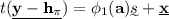. By adaptive smoothness-I, there is at most one $\pi$ so that this holds with short $\underline{\mathbf{x}}$ and non-zero , desired.

• 3. For $(\mathbf{a}, \mathbf{R})\leftarrow \textsf {sim}(1^n)$, $({\pi }, \mathbf{y})\in \mathcal{L}^*$ can be verified using R as follows. For each $t\in \mathbb {Z}_q^*$, try to use R to recover $(s, \mathbf{x})$ so that $t(\mathbf{y}-\mathbf{h}_{\pi })=\mathbf{a}s+\mathbf{x}$ for short $\mathbf{x}$. If it succeeds, then claim $({\pi }, \mathbf{y})\in \mathcal{L}^*$; otherwise, claim $({\pi }, \mathbf{y})\not \in \mathcal{L}^*.$ The validity of this algorithm is by the decoding capability of $\mathbf{R}.$

The commitment security is evident: the hiding property is by the ring-DLWE assumption and the binding property follows from properties 1, 2 above for $\mathcal{L}^*$.

Description of $\delta$-ASPH$_B$. We now define $\mathcal{H}$ and $\hat{\mathcal{H}}$. Take secret $\mathbf{E}$ discrete Gaussian over $\mathbb {Z}^{n\ell \times \mu }$ and the projection key is $\mathbf{U}=\alpha (\mathbf{E}) {=}{} \mathbf{E}^T\phi _1(\mathbf{a})$. The projective hash $\mathcal{H}(\mathbf{E}, {\pi }, \mathbf{y}){=}{} \mathbf{E}^T(\underline{\mathbf{y}-\mathbf{h}_{\pi }}).$ With witness $\tau =(s, \mathbf{x})$, define .

Correctness. For $({\pi }, \mathbf{y})\in \mathcal{L}$, let $\mathbf{y}=\mathbf{a}s+\mathbf{h}_{\pi }+\mathbf{x}$ with short $\underline{\mathbf{x}}$. Then, by Lemma 13(3), The correctness follows as $||\mathbf{E}^T\underline{\mathbf{x}}||_\infty$ is small by Lemma 2 (since $\mathbf{E}$ is Gaussian and $\underline{\mathbf{x}}$ is short).

Smoothness. For any $({\pi }, \mathbf{y})\not \in \mathcal{L}^*$, $\mathbf{y}$ can not be expressed as $t(\mathbf{y}-\mathbf{h}_\pi )=\mathbf{a}s+\mathbf{x}$ with short $\underline{\mathbf{x}}$ for some $(t, s)\ne (0, 0)$. Via Lemma 13(3), is large for any non-zero (t, s). By adaptive smoothness-I, $\mathbf{E}^T(\phi _1(\mathbf{a}), \underline{\mathbf{y}-\mathbf{h}_\pi })$, is close to uniform over $\mathbb {Z}_q^{\mu \times (n+1)}$.

5.4 A Ring-LWE-Based Instantiation of PAKE

We now instantiate our framework from Ring-LWE. In a nutshell, we realize the KF-MAC using the construction in Sect. 3.3 and key reconciliation scheme from Sect. 3.2, while instantiating $\mathbb {H}_1=(\varPi _1, \textsf {ver}^*_1, \mathcal{H}_1, \hat{\mathcal{H}}_1, \alpha _1)$ by $\delta$-ASPH$_B$ and $\mathbb {H}_2=(\varPi _2, \textsf {ver}^*_2, \mathcal{H}_2, \hat{\mathcal{H}}_2, \alpha _2)$ by $\delta$-${\text{ ASPH }}_A$, constructed in the last subsection. Our protocol will use the following parameters, notations and functions.

• m is a power of 2; $n=\frac{m}{2}$; $\theta \in (0, 1)$; prime q; p a constant prime with $p<q$; $\ell _1=\varTheta (\log n)$ and $\ell _2=\omega (1)\le \ell _1$; $k=o(n)$; password dictionary $\mathcal{D}\subseteq \mathbb {Z}_p^k$.

• For $i=1, 2$, let $\mathcal{C}_i$ be a $[\ell _i n, k, \theta \ell _in]_p$-code from Lemma 7.

• $\mathbb {H}_1$ takes $\mathbf{a}, \mathbf{h}\leftarrow R_q^{\ell _1}$ as its public-key and uses code $\mathcal{C}_1$.

• $\mathbb {H}_2$ takes $\mathbf{g}\leftarrow R_q^{\ell _2}, \mathbf{D}=({d}_{ij})\leftarrow R_q^{\ell _2\times 2}$ as its public-key and uses code $\mathcal{C}_2$. In addition, we use $\mathbf{v}=\mathbf{o}^T\mathbf{D} \in R_q^{2}$ with $\mathbf{o}\leftarrow (D_{R, \sqrt{n}r_2})^{\ell _2}$ as the public projection key for the PAKE framework.

• $\delta _1$ is the bound on the noise term for the commitment in $\mathbb {H}_1$ and $\mathbb {H}_2$.

• As before, $F_K$ is the KF-MAC in Sect. 3.3 with a fuzzy verification function $\varPhi _{K'}$; G is a pseudorandom generator; is a reconciliation scheme for Alice and Bob, as in Sect. 3.2.

The public parameter is . Then, the instantiated PAKE protocol between $P_i$ and $P_j$ is described in Fig. 4 (see Sect. 5.4 for details).

Fig. 4.

Our Protocol RLWE-PAKE: $\mathbf{t}\leftarrow R_q^{2}$ and $\mathbf{z}\leftarrow (D_{R, \sqrt{n}r_1})^{\ell _2}$ are sampled with randomness $\varUpsilon$, where $\varUpsilon |sk=G(\varvec{\xi })$.

Fig. 5.

Performance of RLWE-PAKE

5.5 Implementation Results

Due to the space limitation, the efficiency details and comparison are given in the full paper and a summary is given in Table 1. We now provide a proof-of-concept implementation of our RLWE-PAKE scheme. The parameters are chosen as Fig. 5(a) and the output of H is 256 bits. The implementation is done on the platform of Intel Core i7-7700HQ CPU at 2.80 GHz with 7.7 GiB RAM running on the Ubuntu 16.04 LTS 64-bits operation system. Our program uses C++ language and the Number Theory Library (NTL) [27] without parallel techniques. The computational performance is presented in Fig. 5(b). In the setup phase, public parameters are generated. The columns of $P_i$ and $P_j$ denote the time cost of computations by $P_i$ and $P_j$ respectively. The message size and session key size are listed in Fig. 5(c). It shows the message sizes by $P_i$ and $P_j$ respectively in order to agree on a 16 bytes session key. This is a reference implementation without optimizing. Practically, matrix multiplications can be done in parallel.

References

Alwen, J., Peikert, C.: Generating shorter bases for hard random lattices. In: STACS 2009. LIPIcs, vol. 3, pp. 75–86 (2009)
Banaszczyk, W.: Inequalites for convex bodies and polar reciprocal lattices in r\({}^{\text{ n }}\). Discrete Comput. Geom. 13, 217–231 (1995)
Bellare, M., Pointcheval, D., Rogaway, P.: Authenticated key exchange secure against dictionary attacks. In: Preneel, B. (ed.) EUROCRYPT 2000. LNCS, vol. 1807, pp. 139–155. Springer, Heidelberg (2000). https://doi.org/10.1007/3-540-45539-6_11
Bellovin, S.M., Merritt, M.: Encrypted key exchange: password-based protocols secure against dictionary attacks. In: IEEE S&P, pp. 72–84 (1992)
Benhamouda, F., Blazy, O., Ducas, L., Quach, W.: Hash proof systems over lattices revisited. In: Abdalla, M., Dahab, R. (eds.) PKC 2018. LNCS, vol. 10770, pp. 644–674. Springer, Cham (2018). https://doi.org/10.1007/978-3-319-76581-5_22
Canetti, R., Dachman-Soled, D., Vaikuntanathan, V., Wee, H.: Efficient Password Authenticated Key Exchange via Oblivious Transfer. In: Fischlin, M., Buchmann, J., Manulis, M. (eds.) PKC 2012. LNCS, vol. 7293, pp. 449–466. Springer, Heidelberg (2012). https://doi.org/10.1007/978-3-642-30057-8_27
Di Crescenzo, G., Graveman, R., Ge, R., Arce, G.: Approximate message authentication and biometric entity authentication. In: Patrick, A.S., Yung, M. (eds.) FC 2005. LNCS, vol. 3570, pp. 240–254. Springer, Heidelberg (2005). https://doi.org/10.1007/11507840_22
Ding, J., Alsayigh, S., Lancrenon, J., RV, S., Snook, M.: Provably secure password authenticated key exchange based on RLWE for the post-quantum world. In: Handschuh, H. (ed.) CT-RSA 2017. LNCS, vol. 10159, pp. 183–204. Springer, Cham (2017). https://doi.org/10.1007/978-3-319-52153-4_11
Dodis, Y., Goldwasser, S., Tauman Kalai, Y., Peikert, C., Vaikuntanathan, V.: Public-key encryption schemes with auxiliary inputs. In: Micciancio, D. (ed.) TCC 2010. LNCS, vol. 5978, pp. 361–381. Springer, Heidelberg (2010). https://doi.org/10.1007/978-3-642-11799-2_22
Ducas, L., Micciancio, D.: Improved short lattice signatures in the standard model. In: Garay, J.A., Gennaro, R. (eds.) CRYPTO 2014. LNCS, vol. 8616, pp. 335–352. Springer, Heidelberg (2014). https://doi.org/10.1007/978-3-662-44371-2_19
Gennaro, R., Lindell, Y.: A framework for password-based authenticated key exchange. In: Biham, E. (ed.) EUROCRYPT 2003. LNCS, vol. 2656, pp. 524–543. Springer, Heidelberg (2003). https://doi.org/10.1007/3-540-39200-9_33
Gentry, C., Peikert, C., Vaikuntanathan, V.: Trapdoors for hard lattices and new cryptographic constructions. In: STOC 2008, pp. 197–206 (2008)
Goldreich, O., Lindell, Y.: Session-key generation using human passwords only. In: Kilian, J. (ed.) CRYPTO 2001. LNCS, vol. 2139, pp. 408–432. Springer, Heidelberg (2001). https://doi.org/10.1007/3-540-44647-8_24
Gordon, S.D., Katz, J., Vaikuntanathan, V.: A group signature scheme from lattice assumptions. In: Abe, M. (ed.) ASIACRYPT 2010. LNCS, vol. 6477, pp. 395–412. Springer, Heidelberg (2010). https://doi.org/10.1007/978-3-642-17373-8_23
Groce, A., Katz, J.: A new framework for efficient password-based authenticated key exchange. In: CCS 2010, pp. 516–525 (2010)
Jiang, S., Gong, G.: Password based key exchange with mutual authentication. In: Handschuh, H., Hasan, M.A. (eds.) SAC 2004. LNCS, vol. 3357, pp. 267–279. Springer, Heidelberg (2004). https://doi.org/10.1007/978-3-540-30564-4_19
Katz, J., Ostrovsky, R., Yung, M.: Efficient password-authenticated key exchange using human-memorable passwords. In: Pfitzmann, B. (ed.) EUROCRYPT 2001. LNCS, vol. 2045, pp. 475–494. Springer, Heidelberg (2001). https://doi.org/10.1007/3-540-44987-6_29
Katz, J., Vaikuntanathan, V.: Smooth projective hashing and password-based authenticated key exchange from lattices. In: Matsui, M. (ed.) ASIACRYPT 2009. LNCS, vol. 5912, pp. 636–652. Springer, Heidelberg (2009). https://doi.org/10.1007/978-3-642-10366-7_37
Lyubashevsky, V., Peikert, C., Regev, O.: On ideal lattices and learning with errors over rings. J. ACM 60(6), 43:1–43:35 (2013)
Lyubashevsky, V., Peikert, C., Regev, O.: A toolkit for ring-LWE cryptography. In: Johansson, T., Nguyen, P.Q. (eds.) EUROCRYPT 2013. LNCS, vol. 7881, pp. 35–54. Springer, Heidelberg (2013). https://doi.org/10.1007/978-3-642-38348-9_3
Micciancio, D., Peikert, C.: Trapdoors for lattices: simpler, tighter, faster, smaller. In: Pointcheval, D., Johansson, T. (eds.) EUROCRYPT 2012. LNCS, vol. 7237, pp. 700–718. Springer, Heidelberg (2012). https://doi.org/10.1007/978-3-642-29011-4_41
Micciancio, D., Regev, O.: Worst-case to average-case reductions based on Gaussian measures. SIAM J. Comput. 37(1), 267–302 (2007)
Micciancio, D., Walter, M.: Gaussian sampling over the integers: efficient, generic, constant-time. In: Katz, J., Shacham, H. (eds.) CRYPTO 2017. LNCS, vol. 10402, pp. 455–485. Springer, Cham (2017). https://doi.org/10.1007/978-3-319-63715-0_16
Peikert, C.: Lattice cryptography for the internet. In: Mosca, M. (ed.) PQCrypto 2014. LNCS, vol. 8772, pp. 197–219. Springer, Cham (2014). https://doi.org/10.1007/978-3-319-11659-4_12
Peikert, C.: Limits on the hardness of lattice problems in \(\ell _p\) norms. In: CCC 2007 (2007)
Regev, O.: On lattices, learning with errors, random linear codes, and cryptography. J. ACM 56(6), 34:1–34:40 (2009)
Shoup, V.: NTL: a library for doing number theory. https://www.shoup.net/ntl/
Zhang, J., Yu, Y.: Two-round PAKE from approximate SPH and instantiations from lattices. In: Takagi, T., Peyrin, T. (eds.) ASIACRYPT 2017. LNCS, vol. 10626, pp. 37–67. Springer, Cham (2017). https://doi.org/10.1007/978-3-319-70700-6_2
Zhang, J., Yu, Y., Fan, S., Zhang, Z.: Improved lattice-based CCA2-secure PKE in the standard model. IACR Cryptology ePrint 2019:149 (2019)
Acknowledgement
J. He was supported by scholarship from China Scholarship Council (CSC) under Grant No. 201804910203. Wang was supported by National Research Foundation, Prime Minister’s Office, Singapore under its Strategic Capability Research Centres Funding Initiative and Singapore Ministry of Education under Research Grant MOE2016-T2-2-014(S). Nguyen was supported by the Gopalakrishnan-NTU Presidential Postdoctoral Fellowship 2018. Guang Gong’s research is supported by NSERC SPG.
Author information
Authors and Affiliations
Corresponding author
Editor information
Editors and Affiliations
Rights and permissions
Copyright information
© 2020 International Association for Cryptologic Research
About this paper
Cite this paper
Jiang, S., Gong, G., He, J., Nguyen, K., Wang, H. (2020). PAKEs: New Framework, New Techniques and More Efficient Lattice-Based Constructions in the Standard Model. In: Kiayias, A., Kohlweiss, M., Wallden, P., Zikas, V. (eds) Public-Key Cryptography – PKC 2020. PKC 2020. Lecture Notes in Computer Science(), vol 12110. Springer, Cham. https://doi.org/10.1007/978-3-030-45374-9_14
Download citation
DOI: https://doi.org/10.1007/978-3-030-45374-9_14
Published:
Publisher Name: Springer, Cham
Print ISBN: 978-3-030-45373-2
Online ISBN: 978-3-030-45374-9
eBook Packages: Computer ScienceComputer Science (R0)