Statistical Issues in Particle Physics

Abstract

The most exciting result in recent years in Particle Physics was the discovery of the Higgs boson. This involved several interesting statistical issues, which are among those discussed in this article. These include:

• Should we insist on at least a 5σ effect to claim a discovery?

• How should p-values be combined?

• If two different models both have respectable χ ² probabilities, can it be reasonable to reject one in favour of the other?

• Are there different possibilities for quoting the sensitivity of a search?

• How do upper limits change as the number of observed events becomes smaller and smaller than the predicted background?

• Do we really need ‘coverage’?

• Is it possible to combine 1 ± 10 and 2.0 ± 7.5 (two measurements of the same parameter) to obtain a result of 5 ± 1?

• What is the Punzi effect and how can it be understood?

• What checks should be made when Deep Learning techniques are applied to separate signal and background?

15.1 Introduction

In recent years there has been a growing awareness by particle physicists of the desirability of using good statistical practice. This is because the accelerator and detector facilities have become so complex and expensive, and involve so much physicist effort to build, test and run, that it is clearly important to treat the data with respect, and to extract the maximum information from them. The PHYSTAT series of Workshops and Conferences[1,2,3,4,5,6,7,8,9,10,11,12] has been devoted specifically to statistical issues in particle physics and neighbouring fields, and many interesting articles can be found in the relevant Proceedings. These meetings have benefited enormously from the involvement of professional statisticians, who have been able to provide specific advice as well as pointing us to some techniques which had not yet filtered down to Particle Physics analyses.

Analyses of experimental data in Particle Physics have, perhaps not surprisingly, tended to use statistical methods that have been described by other Particle Physicists. There are thus several books written on the subject by Particle Physicists[13]. The Review of Particle Physics properties[14] contains a condensed review of Statistics.

Another source of useful information is provided by the statistics committees set up by some of the large collaborations (see, for example, refs. [15,16,17,18]). Some conferences now include plenary talks specifically on relevant statistical issues (for example, Neutrino 2017[19], NuPhys17 and NuPhys18[20]), and the CERN Summer Schools for graduate students regularly have a series of lectures on statistics for Particle Physics[21].

This article is a slightly updated version of the one that appeared in ref. [22] in 2012.

15.1.1 Types of Statistical Analysis

There are several different types of statistical procedures employed by Particle Physicists:

• Separating signal from background: Almost every Particle Physics analysis uses some method to enhance the possible signal with respect to uninteresting background.

• Parameter determination: Many analyses make use of some theoretical or empirical model, and use the data to determine values of parameters, and their uncertainties and possible correlations.

• Goodness of fit: Here the data are compared with a particular hypothesis, often involving free parameters, to check their degree of consistency.

• Comparing hypotheses: The data are used to see which of two hypotheses is favoured. These could be the Standard Model (SM), and some specific version of new physics such as the existence of SUperSYmmetry (SUSY), or the discovery of the Higgs boson[23].

• Decision making: Based on one’s belief about the current state of physics, the value of possible discoveries and estimates of the difficulty of future experiments, a decision is made on what should be thrust of future research. This subject is beyond the scope of this article.

15.1.2 Statistical and Systematic Uncertainties

In general any attempt to measure a physics parameter will be affected by statistical and by systematic uncertainties. The former are such that, if the experiment were to be repeated, random effects would result in a distribution of results being obtained. These can include effects due to the limited accuracy of the measurement devices and/or the experimentalist; and also from the inherent Poisson variability of observing a number of counts n. On the other hand, there can be effects that shift the measurements from their true values, and which need to be corrected for; uncertainties in these corrections contribute to the systematics. Another systematic effect could arise from uncertainties in theoretical models which are used to interpret the data. Scientists’ systematics are often ‘nuisance parameters’ for statisticians.

Consider an experiment designed to measure the temperature at the centre of the sun by measuring the flux of solar neutrinos on earth. The main statistical uncertainty might well be that due to the limited number of neutrino interactions observed in the detector. On the other hand, there are likely to be systematics from limited knowledge of neutrino cross-sections in the detector material, the energy calibration of the detector, neutrino oscillation parameters, models of energy convection in the sun, etc. If some calibration measurement or subsidiary experiment can be performed, this effectively converts a systematic uncertainty into a statistical one. Whether this source of uncertainty is quoted as statistical or systematic is not crucial; what is important is that possible sources of correlation between uncertainties here and in other measurements (in this or in other experiments) are well understood.

The magnitude of systematic effects in a parameter-determination situation can be assessed by fitting the data with different values of the nuisance parameter(s), and seeing how much the result changes¹ when the nuisance parameter value is varied by its uncertainty. Alternatively the nuisance parameter(s) for systematic effects can be incorporated into the likelihood or χ ² for the fit; or a Bayesian method involving the prior probability distribution for the nuisance parameter can be used. (See Sects. 15.4.5 and 15.7.6 for ways of incorporating nuisance parameters in upper limit and in p-value calculations respectively).

How to assess systematics was much discussed at the first Banff meeting[6] and at PHYSTAT-LHC[24,25,26]. A special session of the recent PHYSTATν meeting at CERN[12] was devoted to systematics. Many reviews of this complex subject exist and can be traced back via ref. [27].

In general, much more effort is involved in estimating systematic uncertainties than for parameter determination and the corresponding statistical uncertainties; this is especially the case when the systematics dominate the statistical uncertainty.

Cowan[35] has considered the effect of having an uncertainty in magnitude of a systematic effect. As Cox has remarked[36], there is a difference in knowing that a correction has almost precisely a 20% uncertainty, or that it is somewhere between 0% and 40%.

15.1.3 Bayes and Frequentism

These are two fundamental approaches to making inferences about parameters or whether data support particular hypotheses. There are also other methods which do not correspond to either of these philosophies; the use of χ ² or the likelihood are examples.

Particle physicists tend to favour a frequentist method. This is because in many cases we really believe that our data are representative as samples drawn according to the model we are using (decay time distributions often are exponential; the counts in repeated time intervals do follow a Poisson distribution; etc.), and hence we want to use a statistical approach that allows the data “to speak for themselves”, rather than our analysis being sensitive to our assumptions and beliefs, as embodied in the assumed Bayesian priors. Bayesians would counter this by remarking that frequentist inference can depend on the reference ensemble, the ordering rule, the stopping rule, etc.

With enough data, the results of Bayesian and frequentist approaches usually tend to agree. However, in smallish data samples numerical results from the two approaches can differ.

15.1.3.1 Probability

There are at least three different approaches to the question of what probability is. The first is the mathematical one, which is based on axioms e.g. it must lie in the range 0–1; the probabilities of an event occurring and of it not occurring add up to 1; etc. It does not give much feeling for what probability is, but it does provide the underpinning for the next two methods.

Frequentists, not surprisingly, define probability in terms of frequencies in a long series of essentially identical repetitions² of the relevant procedure. Thus the probability of the number 5 being uppermost in throws of a die is 1∕6, because that is the fraction of times we expect (or approximately observe) it to happen. This implies that probability cannot be defined for a specific occurrence (Will the first astronaut who lands on Mars return to earth alive?) or for the value of a physical constant (Does Dark Matter contribute more than 25% of the critical density of the Universe?).

In contrast, Bayesians define probability in terms of degree of belief. Thus it can be used for unique events or for the values of physical constants. It can also vary from person to person, because my information may differ from yours. The numerical value of the probability to be assigned to a particular statement is determined by the concept of a ‘fair bet’; if I think the probability (or ‘Bayesian credibility’) of the statement being true is 20%, then I must offer odds of 4-to-1, and allow you to bet in either direction.

This difference in approach to probability affects the way Bayesians and frequentists deal with statistical procedures. This is illustrated below by considering parameter determination.

15.1.3.2 Bayesian Approach

The Bayesian approach makes use of Bayes’ Theorem:

$$\displaystyle \begin{aligned} p(A|B) = p(B|A) \times p(A) / p(B), \end{aligned} $$

(15.1)

where p(A) is the probability or probability density of A, and p(A|B) is the conditional probability for A, given that B has happened. This formula is acceptable to frequentists, provided the probablities are frequentist probabilities. However Bayesians use it with A =  parameter (or hypothesis) and B =  data. Then

$$\displaystyle \begin{aligned} p(parameter|data) \propto p(data|parameter) \times p(parameter), \end{aligned} $$

(15.2)

where the three terms are respectively the Bayesian posterior, the likelihood function and the Bayesian prior. Thus Bayes’ theorem enables us to use the data (as encapsulated in the likelihood) to update our prior knowledge (p(parameter)); the combined information is given by the posterior.

Frequentists object to the use of probability for physical parameters. Furthermore, even Bayesians agree that it is often hard to specify a sensible prior. For a parameter which has been well determined in the past, a prior might be a gamma function or log-normal or a (possibly truncated) Gaussian distribution of appropriate central value and width, but for the case where no useful information is available the choice is not so clear; it is easier to parametrise prior knowledge than to quantify prior ignorance. The ‘obvious’ choice of a uniform distribution has the problem of being not unique (Should our lack of knowledge concerning, for example, the mass of a neutrino m _ν be parametrised by a uniform prior for m _ν or for $m_{\nu }^2$ or for $\log m_{\nu }$, etc?). Also a uniform prior over an infinite parameter range cannot be normalised. For situations involving several parameters, the choice of prior becomes even more problematic.

It is important to check that conclusions about possible parameter ranges are not dominated by the choice of prior. This can be achieved by changing to other ‘reasonable’ priors (sensitivity analysis); or by looking at the posterior when the data has been removed.

15.1.3.3 Frequentist Approach: Neyman Construction

The frequentist way of constructing intervals completely eliminates the need for a prior, and avoids considering probability distributions for parameters. Consider a measurement x which provides information concerning a parameter μ. For example, we could use a month’s data from a large solar neutrino detector (x) to estimate the temperature at the centre of the sun (μ). It is assumed that enough is known about solar physics, fusion reactions, neutrino properties, the behaviour of the detector, etc. that, for any given value of μ, the probability density for every x is calculable. Then for that μ, we can select a region in x which contains, say, 90% of this probability. If we do this for every μ, we obtain a 90% confidence band; it shows the values of x which are likely results³ of the experiment for any μ, assuming the theory is correct (see Fig. 15.1). Then if the actual experiment gives a measurement x ₂, it is merely necessary to find the values of μ for which x ₂ is in the confidence band. This is the Neyman construction.

Fig. 15.1

The Neyman construction for setting a confidence range on a parameter μ. At any value of μ, it is assumed that we know the probability density for obtaining a measured value x. (For example, μ could be the temperature of the fusion reactor at the centre of the Sun, while α is the solar neutrio flux, estimated by operating a large underground solar neutrino detector for 1 month.) We can then choose a region in x which contains, say, 90% of the probability; this is denoted by the solid part of the horizontal line. By repeating this procedure for all possible μ, the band between the curved lines is constructed. This confidence band contains the likely values of x for any μ. For a particular measured value x ₂, the confidence interval from μ _l to μ _u gives the range of parameter values for which that measured value was likely. For x ₂, this interval would be two-sided, while for a lower value x ₁, an upper limit would be obtained. In contrast, there are no parameter values for which x ₀ is likely, and for that measured value the confidence interval would be empty

Of course, the choice of a region in x to contain 90% of the probability is not unique. The one shown in Fig. 15.1 is a central one, with 5% of the probability on either side of the selected region. Another possibility would be to have a region with 10% of the probability to the left, and then the region in x extends up to infinity. This choice would be appropriate if we always wanted to quote upper limits on μ. Other choices of ‘ordering rule’ are also possible (see, for example, Sect. 15.4.3).

The Neyman construction can be extended to more parameters and measurements, but in practice it is very hard to use it when more than two or three parameters are involved; software to perform a Neyman construction efficiently in several dimensions would be very welcome. The choice of ordering rule is also very important. Thus from a pragmatic point of view, even ardent frequentists are prepared to use Bayesian techniques for multidimensional problems (e.g. with systematics). They would, however, like to ensure that the technique they use provides parameter intervals with reasonable frequentist coverage.

15.1.3.4 Coverage

One of the major advantages of the frequentist Neyman construction is that it guarantees coverage. This is a property of a statistical technique⁴ for calculating intervals, and specifies how often the interval contains the true value μ _t of the parameter. This can vary with μ _t.

For example, for a Poisson counting experiment with parameter μ and observed number n, a (not very good) method for providing an interval for μ is $n \pm \sqrt {n}$. Thus an observed n = 2 would give a range 0.59–3.41 for μ. If μ = 2.01, observed values n = 2, 3 and 4 result in intervals that include μ = 2.01, while other values of n do not. The coverage of this procedure for μ = 2.01 is thus the sum of the Poisson probabilities for having n = 2, 3 or 4 for the given μ.

For a discrete observable (e.g. the number of detected events in a search for Dark Matter), there are jumps in the coverage; in order to avoid under-coverage, there is necessarily some over-coverage. However, for a continuous observable (e.g. the estimated mass of the Higgs boson) the coverage can be exact.

Coverage is not guaranteed for methods that do not use the Neyman construction (see Sect. 15.2.1). Interesting plots of coverage as a function of the parameter value for the simple case of a Poisson counting experiment can be found in ref. [32].

15.1.3.5 Likelihoods

The likelihood approach makes use of the probability density function (pdf) for observing the data, evaluated for the data actually observed.⁵ It is a function of any parameters, although it does not behave like a probability density for them. It provides a method for determining values of parameters. These include point estimates for the ‘best’ values, and ranges (or contours in multi-parameter situations) to characterise the uncertainties. It usually has good properties asymptotically, but a major use is with sparse multi-dimensional data.

The likelihood method is neither frequentist nor Bayesian. It thus does not guarantee frequentist coverage or Bayesian credibility. It does, however, play a central role in the Bayesian approach, which obtains the posterior probability density by multiplying the likelihood by the prior. The Bayesian approach thus obeys the likelihood principle, which states that the only way the experimental data affects inference is via the likelihood function. In contrast, the Neyman construction requires not only the likelihood for the actual data, but also for all possible data that might have been observed.

Because the likelihood is not a probability density, it does not transform like one. Thus the value of the likelihood for a parameter μ ₀ is identical to that for λ ₀ = 1∕μ ₀. This means that ratios of likelihoods (or differences in their logarithms) are useful to consider, but that the integration of tails of likelihoods is not a recognised statistical procedure.

A longer account of the Bayesian and frequentist approaches can be found in ref. [28]. Reference [29] provides a very readable account for a Poisson counting experiment.

15.2 Likelihood Issues

In this section, we discuss some potential misunderstandings of likelihoods.

15.2.1 Δ(lnL) = 0.5 Rule

In the maximum likelihood approach to parameter determination, the best value λ ₀ of a parameter is determined by finding where the likelihood maximises; and its uncertainty is estimated by finding how much the parameter must be changed⁶ in order for the logarithm of the likelihood to decrease by 0.5 as compared with the maximum.⁷ From a frequentist viewpoint, this should ideally result in the parameter range having 68% coverage. That is, in repeated use of this procedure to estimate the parameter, 68% of the intervals should contain the true value of the parameter, whatever its true value happens to be.

If the measurement is distributed about the true value as a Gaussian with constant width, the likelihood approach will yield exact coverage, but in general this is not so. For example, Garwood[31] and Heinrich[32] have investigated the properties of the likelihood approach (and other methods too) to estimate μ, the mean of a Poisson, when n _obs events are observed. Because n _obs is a discrete variable, the coverage is a discontinuous function of μ, and varies from 100% at μ = 0 down to 30% at μ ≈ 0.5.⁸

15.2.2 Unbinned Maximum Likelihood and Goodness of Fit

With sparse data, the unbinned likelihood method is a good one for estimating parameters of a model. In order to understand whether these estimates of the parameters are meaningful, we need to know whether the model provides an adequate description of the data. Unfortunately, as emphasised by Heinrich[33], the magnitude of the unbinned maximum likelihood is often independent of whether or not the data agree with the model. He illustrates this by the example of the determination of the lifetime τ of a particle whose decay distribution is (1∕τ)exp(−t∕τ). For a set of observed times t _i, the maximum likelihood L _max depends on the data t _i only through their average value $\bar {t}$. Thus any data distributions with the same $\bar {t}$ would give identical L _max, which demonstrates that, at least in this case, L _max gives no discrimination about whether the data are consistent with the expected distribution.

Another example is fitting an expected distribution $(1 + \alpha \cos ^2\theta )/(1+\alpha /3)$ to data θ _i on the decay angle of some particle, to determine α. According to the expected functional form, the data should be symmetrically distributed about $\cos \theta = 0$. However, the likelihood depends only on the square of $\cos \theta$, and so would be insensitive to all the data having $\cos \theta _i$ negative; this would be very inconsistent with the expected symmetric distribution.

In contrast Baker and Cousins[34] provide a likelihood method of measuring goodness of fit for a data histogram compared to a theory. The Poisson likelihood P _Pois(n|μ) for each bin is compared with that for the best possible predicted value μ _best = n for that bin. Thus the Baker-Cousins likelihood ratio

$$\displaystyle \begin{aligned} LR_{BC} = \Pi \frac{{e^{-\mu_i} \mu_i^{n_i}/n_i!}} {e^{-n_i} n_i^{n_i}/n_i!} = \Pi e^{(n_i - \mu_i)} (\mu_i/n_i)^{n_i} \end{aligned} $$

(15.3)

is such that asymptotically − 2lnLR _BC is distributed as χ ².⁹ For small μ, the Baker-Cousins likelihood ratio is better than a weighted sum of squares for assessing goodness of fit.

15.2.3 Profile Likelihood

In many situations the likelihood is a function not only of the parameter of interest ϕ but also other parameters. These may be other physics parameters (for example, in neutrino oscillation experiments where the mixing angles and differences in mass-squared of the various neutrinos are relevant), but can also be nuisance parameters ν associated with systematic effects (e.g. jet energy scales, particle identification efficiencies, etc.). To make statements about ϕ, the likelihood L(ϕ.ν) is often ‘profiled’ over the nuisance parameters, i.e. at each value of ϕ, the likelihood is remaximised with respect to ν. Thus

$$\displaystyle \begin{aligned} L_{prof} (\phi) = L(\phi, \nu_{max}(\phi)) \end{aligned} $$

(15.4)

Then L _prof(ϕ) is used much as the ordinary likelihood when there are no nuisance parameters.

A profile likelihood is in general wider than the likelihood for a fixed value of the nuisance parameter ν; this results in the uncertainty in the parameter of interest ϕ being larger when allowance is made for the systematic uncertainties.

In the standard profile likelihood, ν is a continuous variable. An extension of this has been used by Dauncey et al. [38], to allow for uncertainties in the choice of functional form of the background parametrisation in searches for new particles as peaks above background in a mass spectrum. Here the systematic is discrete, rather than continuous.

An alternative way of eliminating nuisance parameters (known as marginalisation) is to use L(ϕ, ν) as part of a Bayesian procedure, and than to integrate the Bayesian posterior over ν. i.e.

$$\displaystyle \begin{aligned} P_{marg}(\phi) = \int P_{post}(\phi,\nu) \ d\nu \end{aligned} $$

(15.5)

Of course, both profiling and marginalisation result in the loss of information. Reference [37] provides a very trivial example of this for profile likelihoods.

15.2.4 Punzi Effect

Sometimes we have two or more nearby peaks, and we try to fit our data in order to determine the fractions of each peak. Punzi [39] has pointed out that it is very easy to write down a plausible but incorrect likelihood function that gives a biassed result. This occurs in situations where the events have experimental resolutions σ in the observable x that vary event-by-event; and the distributions of σ are different for the two peaks.

For a set of observations x _i, it is tempting but wrong to write the unbinned likelihood as

$$\displaystyle \begin{aligned} L(f)_{wrong} = \Pi\{f*G(x_i,0.0,\sigma_i) + (1-f) *G(x_i,1.0,\sigma_i)\} \end{aligned} $$

(15.6)

where f is the fraction of the first peak (labelled A below) which is parametrised as G(x _i, 0.0, σ _i), a Gaussian in x _i, centred on zero, and with width σ _i, and i is the label for the ith event; and similarly for the second peak (labelled B), except that it is centred at unity.

Application of the rules of conditional probability shows that the correct likelihood is

$$\displaystyle \begin{aligned} L(f)_{right} =\Pi\{f*G(x_i,0.0,\sigma_i)*p(\sigma_i| A) + (1-f) *G(x_i,1.0,\sigma_i)*p(\sigma_i| B)\} \end{aligned} $$

(15.7)

where p(σ _i|A) and p(σ _i|B) are the probability densities for the resolution being σ _i for the A and B peaks respectively. We then see that L(f)_wrong and L(f)_right give identical values for f, provided that p(σ _i|A) = p(σ _i|B). If however, the distributions of the resolution differ, L(f)_wrong will in general give a biassed estimate.

Punzi investigated the extent of this bias in a simple Monte Carlo simulation, and it turns out to be surprisingly large. For example, with f = 1∕3, and p(σ _A) and p(σ _B) being δ −functions at 1.0 and at 2.0 respectively (i.e. σ = 1 for all A events, and σ = 2 for all B events), the fitted value of f from L(f)_wrong turned out to be 0.65. Given that f is confined to the range from zero to unity, this is an enormous bias.

The way the bias arises can be understood as follows: The fraction f of the events that are really A have relatively good resolution, and so the fit to them alone would assign essentially all of them as belonging to A i.e. these events alone would give f ≈ 1 with a small uncertainty. In contrast the 1 − f of the events that are B have poor resolution, so for them the fit does not mind too much what is the value of f. But the fit uses all the events together, and so assigns a single f to the complete sample; this will be a weighted average of the f values for the A and for the B events. Because the A events result in a more accurate determination of f than do the B events, the fitted f will be biassed upwards (i.e. it will over-estimate the fraction of events corresponding to the peak with the better resolution).

The Punzi effect can also appear in other situations, such as particle identification. Different particle types (e.g. pions and kaons) would appear as different peaks in the relevant particle-identification variable e.g. time of flight, rate of energy loss dE∕dx, angle of Cherenkov radiation, etc. The separation of these peaks for the different particle types depends on the momentum of the particles (see Fig. 15.2). The incorrect L is now

$$\displaystyle \begin{aligned} L_{wrong}(f_K) = \Pi\{(1-f_K) * G(x_i, x_{\pi}(p_i), \sigma_i) + f_K * G(x_i, x_K(p_i), \sigma_i)\} \end{aligned} $$

(15.8)

where x _π(p _i) and x _K(p _i) are the expected positions of the particle identification information for a particle of momentum p _i, and x _i is the observed value for the ith event. So here the Punzi bias can arise even with constant resolution, because the momentum spectra of pions and kaons can be different. To avoid the bias, the likelihood needs to incorporate information on the different momentum distributions of pions and of kaons. If these momentum distributions are different enough from each other, it could be that the likelihood function bases its separation of the different particle types on the momenta of the particles rather than on the data from the detector’s particle identifier. Catastini and Punzi[40] avoid this by using parametric forms for the momentum distributions of the particles, with the parameters being determined by the data being analysed.

Fig. 15.2

The Punzi effect in particle identification. The diagrams show the expected (normalised) distributions of the output signal from a particle identifier, for pions and for kaons (a) at low momentum where separation is easier, and (b) at high momentum where the distributions overlap. Because kaons are heavier than pions, they tend to have larger momenta. Because it is hard at high momentum to distinguish pions from kaons, the likelihood function is insensitive to whether these tracks are classified as pions or kaons, and hence the fraction of high momentum tracks classified as kaons will have a large uncertainty. In contrast, low momentum tracks will be correctly identified. Thus if the plausible but incorrect likelihood function that ignores the pion and kaon momentum distributions is used to determine the overall fraction of kaons, it will be biassed downwards towards the fraction of low momentum particles that are kaons

The common feature potentially leading to bias in these two examples is that the ratio of peak separation to resolution is different for the two types of objects. For the first example of separating the two peaks, it was the denominators that were different, while in the particle identification problem it was the numerators.

The Punzi bias may thus occur in situations where the templates in a multi-component fit depend on additional observations whose distributions are not explicitly included in the likelihood.

15.3 Separating Signal from Background

Almost every Particle Physics analysis uses some technique for separating possible signal from background. First some simple ‘cuts’ are applied; these are generally loose selections on single variables, which are designed to remove a large fraction of the background while barely reducing the real or potential signal. Then to obtain a better separation of signal from background in the multi-dimensional space of the event observables, methods like Fisher discriminants, decision trees, artificial neural networks (including Bayesian nets and more recently deep neural nets), support vector machines, etc. are used[41, 42]. Extensions of these methods involve bagging, boosting and random forests, which have been used to achieve improved performance of the separation as seen on a plot of signal efficiency against background mis-acceptance rate. A description of the software available for implementing some of these techniques can be found in the talks by Narsky[43] and by Tegenfeldt[44] at the PHYSTAT-LHC Workshop.

More recently, deep learning techniques are rapidly becoming popular. In Particle Physics, they have been used for on-line triggering, tracking, fast simulation, object identification, image recognition, and event-by-event separation of signal from background. Reference [45] provides good introductions to the use of these methods for Particle Physics. There are now regular workshops and lectures on Machine Learning at CERN and at Fermilab (see refs. [46] and [47]), as well as at many universities.

The signal-to-background ratio before this multivariate stage can vary widely, as can the signal purity after it. If some large statistics study is being performed (e.g. to use a large sample of events to obtain an accurate measurement of the lifetime of some particle), then it is not a disaster if there is some level of background in the finally selected events, provided that it can be accurately assessed and allowed for in the subsequent analysis. At the other extreme, the separation technique may be used to see if there is any evidence for the existence of some hypothesised particle (the potential signal), in the presence of background from well-known sources. Then the actual data may in fact contain no observable signal.

These techniques are usually ‘taught’ to recognise signal and background by being given examples consisting of large numbers of events of each type. These may be produced by Monte Carlo simulation, but then there is a problem of trying to verify that the simulation is a sufficiently accurate representation of reality. It is better to use real data for this, but the difficulty then is to obtain sufficiently pure samples of background and signal. Indeed, for the search for a new particle, true data examples do not exist. However, it is the accurate representation of background that is likely to pose a more serious problem.

The way that, for example, neural networks are trained is to present the software with approximately equal numbers of signal and background events¹⁰ and then to minimise a cost function C for the network. This is usually defined as C =  Σ(z _i − t _i)², where z _i is the trained network’s output for the ith event; t _i is the target output, usually chosen as 1 for signal and zero for background; and the summation is over all testing events presented to the network. The problem with this is that C is only loosely related to what we really want to optimise. For a search for a new particle this could be the sensitivity of the experimental upper limit in the absence of signal, while for a high statistics analysis measuring the properties (such as mass or lifetime) of some well-established particle, we would be interested in minimising the uncertainty (including systematic effects) on the result, without the training procedure biassing the measurement.

As with all event separation methods. it is essential to check the performance of a trained procedure by using a set of events that are independent of those used for training. This is to ensure that the network does not use specific but irrelevant features of the training events in its learning process, but can achieve good performance on unseen data.

Some open questions are:

• How can we check that our multi-dimensional training samples for signal and background are reliable descriptions of reality; and that they cover the region of multi-dimensional space populated by the data?

• How should the ratio of the numbers of signal and background training events be chosen, especially when there are several different sources of background?

• What is the best way of allowing for nuisance parameters in the models of the signal and/or background?[25, 48]

• Are there useful and easy ways of optimising on what is really of interest?[49]

15.3.1 Understanding How Neural Networks Operate

It is useful to appreciate how neural networks operate in providing a good separation of signal and background, as this can help in choosing a suitable architecture for the network.

Figure 15.3a shows some hypothetical signal and background events in terms of two measured variables x and y for each event. A network with two inputs (x and y), a single hidden layer with 3 nodes, and a single output is used; it aims to give 1 for signal and zero for background events (see Fig. 15.3b. This is achieved by training the network with (x, y) values for known examples of signal and background; and allowing the network to vary its internal parameters to minimise a suitably defined cost function e.g. Σ(z _e − t _e)², where the summation is over the training events, and z _e and t _e are the network’s output and its target value (0 or 1) respectively.

Fig. 15.3

(a) A 2 − D plot showing the regions of the variables v ₁ and v ₂ for the signal (dots)and background (triangles). (b) The neural network used for separating signal and background. (c) The top hidden node receives inputs from v ₁ and v ₂. With suitable weights and threshold and a large value of β, the node’s output will be on for (v ₁, v ₂) values below the diagonal line. (d) Similarly for the other two hidden nodes, their outputs can be on for (v1, v2) below the other diagonal line, and above the horizontal one, respectively. A further choice of weights to the output node and its threshold can ensure that the whole network’s output will be on only if all three hidden nodes’ outputs are on, i.e. if (v ₁, v ₂) values are within the triangle in (d)

The input q _i to a given hidden node i is a linear combination of the input variables x and y

$$\displaystyle \begin{aligned} q_i = w_{xi}x + w_{yi}y + t_i \end{aligned} $$

(15.9)

where the weights w and threshold t are varied during the fitting process. The output r from any hidden node is determined from its input q by something like a sigmoid function e.g.

$$\displaystyle \begin{aligned} r = 1/(1+e^{-\beta q}) \end{aligned} $$

(15.10)

This switches from zero for large negative q to unity for large positive q. The switch occurs around q = 0, and width of the region depends on the network parameter β. For very large β, there is a rapid switch from zero to unity. In terms of x and y, this means that the hidden node i is ‘on’ (i.e. r _i = 1) if

$$\displaystyle \begin{aligned} w_{xi}x + w_{yi}y +t_i > 0, \end{aligned} $$

(15.11)

or ‘off’ otherwise. Thus the boundary between events having r _i on or off is a straight line in the (x, y) plane (see Fig. 15.3c). With suitable values for the weights and thresholds for the three hidden nodes, there will be three straight line boundaries in the (x, y) plane shown in Fig. 15.3d. Finally, to produce the “and” of these three conditions, the weights w _jo (from the hidden node j to the output node o) and the output threshold t _o can be set as

$$\displaystyle \begin{aligned} w_{1o} = w_{2o} = w_{3o} = 0.4 \ \ \ \ \ \ t_o = -1.0 \end{aligned} $$

(15.12)

to ensure that the output will be “on” only if the three hidden layers are all “on”, i.e. that the selected input values are inside the triangular region in the (x.y) plane. With β set at a lower level, the contour for the selected region will be smoother with rounded corners, rather than being triangular.

It would be useful to have a similar understanding of how deep networks operate. Tishby[50] has provided some insight on what happens in the hidden layers of a deep neural network during the training procedure.

15.4 Parameter Determination

For a single parameter (e.g. the branching ratio for H → μ ⁺μ ⁻) the parameter range could be either a 2-sided interval or just an upper limit, at some confidence level (typically 68% for 2-sided intervals, but usually 90% and 95% for upper limits). For two parameters (e.g. mass and production rate for some new particle X that decays to a top pair), their acceptable values could be those inside some 2-dimensional confidence region. Alternatively an upper limit or 2-sided region for one parameter as a function of the other could be defined; these are known as a Raster Scan.

An upper limit on 2-variables is not a well-defined concept.

15.4.1 Upper Limits

Most recent searches for new phenomena have not found any evidence for exciting new physics. Examples from particle physics include searches for SUSY particles, dark matter, etc.; attempts to find substructure of quarks or leptons; looking for extra spatial dimensions; measuring the mass of the lightest neutrino; etc. Rather than just saying that nothing was found, it is more useful to quote an upper limit on the sought-for effect, as this could be useful in ruling out some theories. For example in 1887, Michelson and Morley[52] attempted to measure the speed of the Earth with respect to the aether. No effect was seen, but the experiment was sensitive enough to lead to the demise of the aether theory.

A simple scenario is a counting experiment where a background b is expected from conventional sources, together with the possibility of an interesting signal s. The number of counts n observed is expected to be Poisson distributed with a mean μ = 𝜖s + b, where b is the expected number of events from background, and 𝜖 is a factor for converting the basic physics parameter s into the number of signal events expected in our particular experiment; it thus allows for experimental inefficiency, the experiment’s running time; etc. Then given a value of n which is comparable to the expected background, what can we say about s? The true value of the parameter s is constrained to be non-negative. The problem is interesting enough if b and 𝜖 are known exactly; it becomes more complicated when only estimates with uncertainties σ _b and σ _𝜖 are available.

An extension of the simple counting scenario is when a search for a new particle is carried out over a range of masses. This is usually dealt with by performing separate searches at a series of masses over a specified range. This ‘Raster Scan’ is in contrast with a method that regards the sought-for new particle’s mass and its production rate as two parameters to be estimated simultaneously. The relative merits of these two approaches are described in ref. [51].

Even without the nuisance parameters, a variety of methods is available. These include likelihood, χ ², Bayesian with various priors for s, frequentist Neyman constructions with a variety of ordering rules for n, and various ad hoc approaches. The methods give different upper limits for the same data.¹¹A comparison of several methods can be found in ref. [53]. The largest discrepancies arise when the observed n is less than the expected background b, presumably because of a downward statistical fluctuation. The following different behaviours of the limit (when n < b) can be obtained:

• Frequentist methods can give empty intervals for s i.e. there are no values of s for which the data are likely. Particle physicists tend to be unhappy when their years of work result in an empty interval for the parameter of interest, and it is little consolation to hear that frequentist statisticians are satisfied with this feature, as it does not necessarily lead to undercoverage.

  When n is not quite small enough to result in an empty interval, the upper limit might be very small.¹² This could confuse people into thinking that the experiment was much more sensitive than it really was.

• The Feldman-Cousins frequentist method[54] (see Sect. 15.4.3) that employs a likelihood-ratio ordering rule gives upper limits which decrease as n gets smaller at constant b. A related effect is the growth of the limit as b decreases at constant n—this can also occur in other frequentist approaches. Thus if no events are observed (n = 0), the upper limit of a 90% Feldman-Cousins interval is 1.08 for b = 3.0, but 2.44 for b = 0. This is sometimes presented as a paradox, in that if a bright graduate student worked hard and discovered how to eliminate the expected background without much reduction in signal efficiency, the ‘reward’ would be a weaker upper limit.¹³ An answer is that although the actual limit had increased, the sensitivity of the experiment with the smaller background was better. There are other situations—for example, variants of the random choice of voltmeter (compare ref. [55])—where a measurement with better sensitivity can on occasion give a less precise result.

• In the Bayesian approach, the dependence of the limit on b is weaker. Indeed when n = 0, the limit does not depend on b.

• Sen et al. [56] consider a related problem, of a physical non-negative parameter λ producing a measurement x, which is distributed about λ as a Gaussian of variance σ ². As the observable x becomes more and more negative, the upper limit on λincreases, because it is deduced that σ must in fact be larger than its quoted value.

In trying to assess which of the methods is best, one first needs a list of desirable properties. These include:

• Coverage: Even though coverage is a frequentist concept, most Bayesian particle physicists would like the coverage of their intervals to match their reported credibility, at least approximately.

  Because the data in counting experiments is discrete, it is impossible in any sensible way to achieve exact coverage for all μ (see Sect. 15.1.3.4). However, it is not completely obvious that even Frequentists need coverage for every possible value of μ, since different experiments will have different values of b and of 𝜖. Thus even for a constant value of the physical parameter s, different experiments will have different μ = 𝜖 ∗ s + b. Thus it would appear that, if coverage in some average (over μ) sense were satisfactory, the frequentist requirement for intervals to contain the true value at the requisite rate would be maintained. This, however, is not the generally accepted view by particle physicists, who would like not to undercover for anyμ.

• Not too much overcoverage: Because coverage varies with μ, for methods that aim not to undercover anywhere, some overcoverage is inevitable. This corresponds to having some upper limits which are high, and this leads to undesirable loss of power in rejecting alternative hypotheses about the parameter’s value.

• Short and empty intervals: These can be obtained for certain values of the observable, without resulting in undercoverage. They are generally regarded as undesirable for the reasons explained above.

It is not obvious how to incorporate the above desiderata on interval length into an algorithm that would be useful for choosing among different methods for setting limits. For different experiments studying the same phenomena (e.g. Dark Matter searches, neutrino oscillation experiments, etc.) it is worthwhile to use the same technique for calculating allowed parameter ranges.

15.4.2 Two-Sided Intervals

An alternative to giving upper limits is to quote two-sided intervals. For example, a 68% confidence interval for the mass of the top quark might be 172.6–173.4 GeV/c ², as opposed to its 95% upper limit being 173.6 GeV/c ². Most of the difficulties and ambiguities mentioned above apply in this case too, together with some extra possibilities. Thus, while it is clear which of two possible upper limits is tighter, this is not necessarily so for two-sided intervals, where which is shorter may be metric dependent; the first of two intervals for a particle’s lifetime τ may be shorter, but the second may be shorter when the ranges are quoted for its decay rate (= 1∕τ). There is also scope for choice of ordering rule for the frequentist Neyman construction, or for choosing the interval from the Bayesian posterior probability density.¹⁴

15.4.3 Feldman-Cousins Approach

Feldman and Cousins’ fully frequentist approach[54] exploits the freedom available in the Neyman construction of how to choose an interval in the data that contains a given fraction α of the probability, by using their ‘ordering rule’. This is based on the likelihood ratio L(x, μ)∕L(x, μ _best), where μ _best is the physically-allowed value of μ which gives the largest value of L for that particular x. For values of μ far from a physical boundary, this makes little difference from the standard central Neyman construction, but near a boundary the region is altered in such a way as to make it unlikely that there will be zero-length or empty intervals for the parameter μ; these can occur in the standard Neyman construction (see Fig. 15.4).

Fig. 15.4

The Feldman-Cousins 90% confidence band (solid curves) for the mean μ of a Gaussian probability density function of unit variance for a measurement x. The straight dashed lines show the confidence band for the central Neyman construction. The Feldman-Cousins ordering rule pulls the interval to the left at small μ, and hence, even for negative observed x, the μ interval is not empty, as happens for central frequentist intervals when x is below − 1.6

The original Feldman-Cousins paper also considered how to extend their method when there is more than one parameter and one measurement. They describe an idealised neutrino oscillation experiment with the data being the energy spectrum of the interacting neutrinos, and the parameters are $\sin ^2(2\theta )$ and Δm ² (see Eq. 15.15). A practical problem of having many parameters is the CPU time required to compute the results.

Feldman and Cousins also point out that an apparently innocuous procedure for choosing what result to quote may lead to undercoverage. Many physicists would quote an upper limit on any possible signal if their observation was less than 3 standard deviations above the expected background, but a two-sided interval if their result was above this. With each type of interval constructed to give 90% coverage, there are some values of the parameter for which the coverage for this mixed procedure drops to 85%; Feldman and Cousins refer to this as ‘flip-flop’. Their ‘unified’ approach circumvents this problem, as it automatically yields upper limits for small values of the data, but two-sided intervals for larger measurements, while avoiding undercoverage for all possible true values of the signal.

15.4.4 Sensitivity

It is useful to quote the sensitivity of a procedure, as well as the actual upper limit as derived from the observed data.¹⁵ For upper limits or for uncertainties on measurements, this can be defined as the median value that would be obtained if the procedure was repeated a large number of times.¹⁶ Using the median is preferable to the mean because (a) it is metric independent (i.e. the median lifetime upper limit would be the reciprocal of the median decay rate lower limit); and (b) it is much less sensitive to a few anomalously large upper limits or uncertainty estimates.

It is common to present not only the median of the expected distribution, but also values corresponding to 16th and 84th percentiles (commonly referred to as ± 1 σ) and also the 2.5% and 97.5% ones (± 2σ). This enables a check to be made that the observed result is reasonable.

Punzi [57] has drawn attention to the fact that this choice of definition for sensitivity has some undesirable features. Thus designing an analysis procedure to minimise the median upper limit for a search in the absence of a signal provides a different optimisation from maximising the median number of standard deviations for the significance of a discovery when the signal is present. Also there is only a 50% chance of achieving the median result or better. Instead, for pre-defined levels α and confidence level CL, Punzi determines at what signal strength there is a probability of at least CL for establishing a discovery at a significance level α. This is what he quotes as the sensitivity, and is the signal strength at which we are sure to be able either to claim a discovery or to exclude its existence. Below this, the presence or otherwise of a signal makes too little difference, and we may remain uncertain (see Fig. 15.5).

Fig. 15.5

Punzi definition of sensitivity. Expected distributions for a statistic t (which in simple cases could be simply the observed number of events n), for H ₀ =  background only (solid curves) and for H ₁ =  background plus signal (dashed curves). In (a), the signal strength is very weak, and it is impossible to choose between H ₀ and H ₁. As shown in (b), which is for moderate signal strength, p ₀ is the probability according to H ₀ of t being equal to or larger than the observed t ₀. To claim a discovery, p ₀ should be smaller than some pre-set level α, usually taken to correspond to 5σ; t _crit is the minimum value of t for this to be so. Similarly p ₁ is the probability according to H ₁ for t ≤ t ₀. The power function is the probability according to the alternative hypothesis that t will exceed t _crit. As the separation of the H ₀ and H ₁pdfs increases, so does the power. According to Punzi, the sensitivity should be defined as the expected production strength of the signal such that the power exceeds another predefined CL, e.g. 95%. The exclusion region corresponds to t ₀ in the 5% lower tail of H ₁, while the discovery region has t ₀ in the 5σ upper tail of H ₀; in (b) there is a “No decision” region in between, as the signal strength is below the sensitivity value. The sensitivity is thus the signal strength above which there is a 95% chance of making a 5σ discovery. i.e. The distributions for H ₀ and H ₁ are sufficiently separated that, apart possibly for the 5σ upper tail of H ₀ and the 5% lower tail of H ₁, they do not overlap. In (c) the signal strength is so large that there is no ambiguity in choosing between the hypotheses

15.4.5 Nuisance Parameters

For calculating upper limits in the simple counting experiment described in Sect. 15.4.1, the nuisance parameters arise from the uncertainties in the background rate b and the acceptance 𝜖. These uncertainties are usually quoted as σ _b and σ _𝜖 (e.g. b = 3.1 ± 0.5), and the question arises of what these uncertainties mean. Sometimes they encapsulate the results of a subsidiary measurement, performed to estimate b or 𝜖, and then they would express the width of the Bayesian posterior or of the frequentist interval obtained for the nuisance parameters. However, in many situations, the uncertainties may involve Monte Carlo simulations, which have systematic uncertainties (e.g. related to how well the simulation describes the real data) as well as statistical ones; or they may reflect uncertainties or ambiguities in theoretical calculations required to derive b and/or 𝜖. In the absence of further information the posterior is often assumed to be a Gaussian, usually truncated so as to exclude unphysical (e.g. negative) values. This may be at best only approximately true, and deviations are likely to be most serious in the tails of the distribution. A log-normal or gamma function may be a better choice.

There are many methods for incorporating nuisance parameters in upper limit calculations. These include:

• Profile likelihood (see also Sect. 15.2.3)

  The likelihood, based on the data from the main and from the subsidiary measurements, is a function of the parameter of interest s and of the nuisance parameters. The profile likelihood L _prof(s) is simply the full likelihood L(s, b _best(s), 𝜖 _best(s)), evaluated at the values of the nuisance parameters that maximise the likelihood at each s. Then the profile likelihood is simply used to extract the limits on s, much as the ordinary likelihood could be used for the case when there are no nuisance parameters.

  Rolke et al. [59] have studied the behaviour of the profile likelihood method for limits. Heinrich[32] had shown that the likelihood approach for estimating a Poisson parameter (in the absence of both background and of nuisance parameters) can have poor coverage at low values of the Poisson parameter. However, the profile likelihood seems to do better, probably because the nuisance parameters have the effect of smoothing away the fluctuating coverage observed by Heinrich.

• Fully Bayesian

  When there is a subsidiary measurement for a nuisance parameter, a prior is chosen for b (or 𝜖), the data are used to extract the likelihood, and then Bayes’ Theorem is used to deduce the posterior for the nuisance parameter. This posterior from the subsidiary measurement is then used as the prior for the nuisance parameter in the main measurement (this prior could alternatively come from information other than a subsidiary measurement); with the prior for s and the likelihood for the main measurement, the overall joint posterior for s and the nuisance parameter(s) is derived.¹⁷ This is then integrated over the nuisance parameter(s) to determine the posterior for s, from which an upper limit can be derived; this procedure is known as marginalisation.

  Numerical examples of upper limits can be found in ref. [60], where a method is discussed in detail. Thus assuming (somewhat unrealistically) precisely determined backgrounds, the effect of a 10% uncertainty in 𝜖 can be seen for various measured values of n in Table 15.1. A plot of the coverage when the uncertainty in 𝜖 is 20% is reproduced in Fig. 15.6.

  Fig. 15.6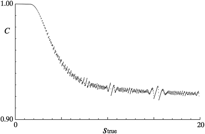

  

  The coverage C for the 90% confidence level upper limit as a function of the true parameter s _true, as obtained in a Bayesian approach. The background b = 3.0 is assumed to be known exactly, while the subsidiary measurement for 𝜖 gives a 20% accuracy. The discontinuities are a result of the discrete (integer) nature of the measurements. There is no undercoverage

  Table 15.1 Bayesian 90% confidence level upper limits for the production rate s as a function of n, the observed number of events

  It is not universally appreciated that the choice for the main measurement of a truncated Gaussian prior for 𝜖 and an (improper) constant prior for non-negative s results in a posterior for s which diverges[61]. Thus numerical estimates of the relevant integrals are meaningless. Another problem comes from the difficulty of choosing sensible multi-dimensional priors. Heinrich has pointed out the problems that can arise for the above Poisson counting experiment, when it is extended to deal with several data channels simultaneously[62].

• Fully frequentist

  In principle, the fully frequentist approach to setting limits when provided with data from the main and from subsidiary measurements is straightforward: the Neyman construction is performed in the multidimensional space where the parameters are s and the nuisance parameters, and the data are from all the relevant measurements. Then the region in parameter space for which the observed data was likely is projected onto the s-axis, to obtain the confidence region for s.

  In practice there are formidable difficulties in writing a program to do this in a reasonable amount of time. Another problem is that, unless a clever ordering rule is used for producing the acceptance region in data space for fixed values of the parameters, the projection phase leads to overcoverage, which can become larger as the number of nuisance parameters increases. Good ordering rules have been found for a version of the Poisson counting experiment[63], and also for the ratio of Poisson means[64], where the confidence intervals are tighter than those obtained by conditioning on the sum of the numbers of counts in the two observations.

  For the fully frequentist method, it is guaranteed that there will be no undercoverage for any combination of parameter true values. This is not so for any other method, and so most particle physicists would like assurance that the technique used does indeed provide reasonable coverage, at least for s. There is usually lively debate between frequentists and Bayesians as to whether coverage is desirable for all values of the nuisance parameter(s), or whether one should be happy with no or little undercoverage when experiments are averaged, for example, over the nuisance parameter true values.

• Mixed

  Because of the difficulty of performing a fully frequentist analysis in all but the simplest problems, an alternative approach[65] is to use Bayesian averaging over the nuisance parameters, but then to employ a frequentist approach for s. The hope is that for most experiments setting upper limits, the statistical uncertainties on the low n data are relatively large and so, provided the uncertainties in the nuisance parameters are not too large, the effect of the systematics on the upper limits will not be too dramatic, and an approximate method of dealing with them may be reasonable.

  Although such an approach cannot be justified from fundamentals, it provides a practical method whose properties can be checked, and is often satisfactory.

15.4.6 Banff Challenges

Given the large number of techniques available for extracting upper limits from data, especially in the presence of nuisance parameters, it was decided at the Banff meeting[6] that it would be useful to compare the properties of the different approaches under comparable conditions. This led to the setting up of the ‘Banff Challenge’, which consisted of providing common data sets for anyone to calculate their upper limits. This was organised by Joel Heinrich, who reported on the performance of the various methods at the PHYSTAT-LHC meeting[66].

At the second Banff meeting[8], the challenge was set by Tom Junk and consisted of participants trying to distinguish between histograms, some of which contained only background and others which contained a background and signal, which appeared as a peak (compare Sect. 15.7.5)

15.4.7 Recommendations

It would be incorrect to say that there is one method that must be used. Many Particle Physicists’ ideal would be to use a frequentist approach if viable software were available for problems with several parameters and items of data. Otherwise they would be prepared to settle for a Bayesian approach, with studies of the sensitivity of the upper limit to the choice of priors, and of the coverage; or for a profile likelihood method, again with coverage studies. What is important is that the procedure should be fully defined before the data are analysed; and that when the experimental result and the sensitivity of the search are reported, the method used should be fully explained.

The CDF Statistics Committee [67] also suggests that it is useful to use a technique that has been employed by other experiments studying the same phenomenon; this makes for easier comparison. They tend to favour a Bayesian approach, chiefly because of the ease of incorporating nuisance parameters.

15.5 Combining Results

This section deals with the combination of the results from two or more measurements of a single (or several) parameters of interest. It is not possible to combine upper limits (UL). This is because an 84% UL of 1.5 could come from a measurement of 1.4 ± 0.1, or 0.5 ± 1.0; these would give very different results when combined with some other measurement.

The combination of p-values is discussed in Sect. 15.7.9.

15.5.1 Single Parameter

An interesting question is whether it is possible to combine two measurements of a single quantity, each with uncertainty ± 10, such that the uncertainty on the combined best estimate is ± 1? The answer can be deduced later.

To combine N different uncorrelated measurements a _i ± σ _i of the same physical quantity a ¹⁸ when the measurements are believed to be Gaussian distributed about the true value a _true, the well-known result is that the best estimate a _comb ± σ _comb is given by

$$\displaystyle \begin{aligned} a_{comb} = \Sigma(a_i * w_i)/\Sigma w_i,\ \ \ \ \ \sigma _{comb} = 1/\sqrt{\Sigma w_i}, \end{aligned} $$

(15.13)

where the weights are defined as $w_i=1/\sigma _i^2$. This is readily derived from minimising with respect to a a weighted sum of squared deviations

$$\displaystyle \begin{aligned} S(a) = \Sigma(a_i - a)^2/\sigma _i^2 \end{aligned} $$

(15.14)

The extension to the case where the individual measurements are correlated (as is often the case for analyses using different techniques on the same data) is straightforward: S(a) becomes Σ Σ(a _i − a) ∗ H _ij ∗ (a _j − a), where H is the inverse covariance matrix for the a _i. It provides Best Linear Unbiassed Estimates (BLUE)[70].

There are, however, practical details that complicate its application. For example, in the above formula, the σ _i are supposed to be the true accuracies of the measurements. Often, all that we have available are estimates of their values. Problems arise in situations where the uncertainty estimate depends on the measured value a _i. For example, in counting experiments with Poisson statistics, it is typical to set the uncertainty as the square root of the observed number. Then a downward fluctuation in the observation results in an overestimated weight, and a _comb is biassed downwards. If instead the uncertainty is estimated as the square root of the expected number a, the combined result is biassed upwards—the increased uncertainty reduces S at larger a. A way round this difficulty has been suggested by Lyons et al. [71]. Alternatively, for Poisson counting data a likelihood approach is preferable to a χ ²-based method.

Another problem arises when the individual measurements are very correlated. When the correlation coefficient of two uncertainties is larger than σ ₁∕σ ₂ (where σ ₁ is the smaller uncertainty), a _comb lies outside the range of the two measurements. As the correlation coefficient tends to +1, the extrapolation becomes larger, and is sensitive to the exact values assumed for the elements of the covariance matrix. The situation is aggravated by the fact that σ _comb tends to zero. This is usually dealt with by selecting one of the two analyses, rather than trying to combine them. However, if the estimated uncertainty increases with the estimated value, choosing the result with the smaller estimated uncertainty can again produce a downward bias. On the other hand, using the smaller expected uncertainty can cause us to ignore an analysis which had a particularly favourable statistical fluctuation, which produced a result that was genuinely more precise than expected¹⁹ How to deal with this situation in general is an open question. It has features in common with the problem (inspired by ref. [55]) of measuring a voltage by choosing at random a voltmeter from a cupboard containing meters of different sensitivities.

Another example involves combining two measurements of a cross-section with small statistical uncertainties, but with large correlated uncertainties from the common luminosity. With this luminosity uncertainty included in the covariance matrix, BLUE can result in the combined value being outside the range of the individual measurements. For this situation, it is preferable to exclude the luminosity uncertainty from the covariance matrix, and to apply it to the combined result afterwards.

15.5.2 Two or More Parameters

An extension of this procedure is for combining N pairs of correlated measurements (e.g. the gradient and intercept of a straight line fit to several sets of data, where for simplicity it is assumed that any pair is independent of every other pair). For several pairs of values (a _i, b _i) with inverse covariance matrices M _i, the best combined values (a _comb, b _comb) have as their inverse covariance matrix M =  ΣM _i. This means that, if the covariance matrix correlation coefficients ρ _i of the different measurements are very different from each other, the uncertainty on a _comb can be much smaller than that for any single measurement.

This situation applies for track fitting to hits in a series of groups of tracking chambers, where each set of close chambers provides a very poor determination of the track; but the combination involves widely spaced chambers and determines the track well. Using the profile likelihoods (e.g. for the intercept, profiled over the gradient) for combining different measurements loses the correlation information and can lead to a very poor combined estimate[37]. The alternative of ignoring the correlation information is also strongly discouraged.

The importance of retaining covariances is relevant for many combinations, e.g. for the determination of the amount of Dark Energy in the Universe from various cosmological data[73].

15.5.3 Data Consistency

The standard procedure for combining data pays no attention to whether or not the data are consistent. If they are clearly inconsistent, then they should not all be combined. When they are somewhat inconsistent, the procedure adopted by the Particle Data Group[14] is to increase all the uncertainties by a common factor such that the overall χ ² per degree of freedom equals unity.²⁰

The Particle Data Group prescription for expanding uncertainties in the case of discrepant data sets has complications when each of the data sets consists of two or more parameters[72].

15.6 Goodness of Fit

15.6.1 Sparse Multi-Dimensional Data

The standard method loved by most scientists uses the weighted sum of squares, commonly called χ ². This, however, is only applicable to binned data (i.e. in a one or more dimensional histogram). Furthermore it loses its attractive feature that its distribution is model-independent when there is not enough data, which is likely to be so in the multi-dimensional case.

Although the maximum likelihood method is very useful for parameter determination with unbinned data, the value of L _max usually does not provide a measure of goodness of fit (see Sect. 15.2.2).

An alternative that is used for sparse one-dimensional data is the Kolmogorov-Smirnov (KS) approach[68], or one of its variants. However, in the presence of fitted parameters, simulation is again required to determine the expected distribution of the KS-distance. Also because of the problem of how to order the data, the way to use it in multi-dimensional situations is not unique.

The standard KS method uses the maximum deviation between two cumulative distributions; because of statistical fluctuations, this is likely to occur near the middle of the distributions. In cases where interesting New Physics is expected to occur at extreme values of some kinematic variable (e.g. p _T), variants of KS such as Anderson-Darling[69] that give extra weight to the distributions’ tails may be more useful.

15.6.2 Number of Degrees of Freedom

If we construct the weighted sum of squares S between a predicted theoretical curve and some data in the form of a histogram, provided the Poisson distribution of the bin contents can be approximated by a Gaussian (and the theory is correct, the data are unbiased, the uncertainty estimates are correct, etc.), asymptotically ²¹S will be distributed as χ ² with the number of degrees of freedom ν = n − f, where n is the number of data points and f is the number of free parameters whose values are determined by minimising S.

The relevance of the asymptotic requirement can be seen by imagining fitting a more or less flat distribution by the expression N(1 + 10⁻⁶cos(x − x ₀)), where the free parameters are the normalisation N and the phase x ₀. It is clear that, although x ₀ is left free in the fit, because of the 10⁻⁶ factor, it will have a negligible effect on the fitted curve, and hence will not result in the typical reduction in S associated with having an extra free parameter. Of course, with an enormous amount of data, we would have sensitivity to x ₀, and so asymptotically it does reduce ν by one unit, but not for smaller amounts of data.

Another example involves neutrino oscillation experiments[54]. In a simplified two neutrino scenario, the neutrino energy spectrum is fitted by a survival probability P of the form

$$\displaystyle \begin{aligned} P = 1 - \sin^2 2\theta\, \sin^2(C* \Delta m^2) , \end{aligned} $$

(15.15)

where C is a known function of the neutrino energy and the length of its flight path, Δm ² is the difference in mass squared of the relevant neutrino species, and θ is the neutrino mixing angle. For small values of C ∗ Δm ², this reduces to

$$\displaystyle \begin{aligned} P \approx 1 - \sin^2 2\theta\, (C* \Delta m^2)^2 \end{aligned} $$

(15.16)

Thus the survival probability depends on the two parameters only via their product $\sin 2\theta \, \Delta m^2$. Because this combination is all that we can hope to determine, we effectively have only one free parameter rather than two. Of course, an enormous amount of data can manage to distinguish between $\sin {}(C* \Delta m^2)$ and C ∗ Δm ², and so asymptotically we have two free parameters as expected.

15.7 Discovery Issues

Searches for new particles are an exciting endeavour, and continue to play a large role at the LHC at CERN, in neutrino experiments, in searches for dark matter, etc. The 2007 and 2011 PHYSTAT Workshops at CERN[7, 9] were devoted specifically to statistical issues that arise in discovery-orientated analyses at the LHC. Ref [74] deals with statistical issues that occur in Particle Physics searches for new phenomena; as an example, it includes the successful search for the Higgs boson at the LHC. A more detailed description of the plans for the Higgs search before its discovery is in ref. [75].

15.7.1 H ₀, or H ₀ Versus H ₁?

In looking for new physics, there are two distinct types of approach. We can compare our data just with the null hypothesis H ₀, the SM of Particle Physics; alternatively we can see whether our data are more consistent with H ₀ or with an alternative hypothesis H ₁, some specific manifestation of new physics, such as a particular form of quark and/or lepton substructure. The former is known as ‘goodness of fit’, while the term ‘hypothesis testing’ is often reserved for the latter.

Each of these approaches has its own advantage. By not specifying a specific alternative,²² the goodness of fit test may be capable of detecting any form of deviation from the SM. On the other hand, if we are searching for some specific new effect, a comparison of H ₀ and H ₁ is likely to be a more sensitive way for that particular alternative. Also, the ‘hypothesis testing’ approach is less likely to give a false discovery claim if the assumed form of H ₀ has been slightly mis-modelled.

15.7.2 p-Values

In order to quantify the chance of the observed effect being due to an uninteresting statistical fluctuation, some statistic is chosen for the data. The simplest case would be the observed number n ₀ of interesting events. Then the p-value is calculated, which is simply the probability that, given the expected background rate b from known sources, the observed value would fluctuate up to n ₀ or larger. In more complicated examples involving several relevant observables, the data statistic may be a likelihood ratio L ₀∕L ₁ for the likelihood of the null hypothesis H ₀ compared with that for a specific alternative H ₁.

To compute the p-value of the observed or of possible data, the distribution f(t) of the data statistic t under the relevant hypothesis is required. In some cases this can be obtained analytically, but in more complicated situations, f(t) may require simulation. For t being − 2lnL ₀∕L _best, Cowan et al have given useful asymptotic formulae for f(t)[76]; here L _best is the value of the likelihood when the parameters in H ₀ are set at their best values.

A small value of p indicates that the data are not very compatible with the theory (which may be because the detector’s response or the background is poorly modeled, rather than the theory being wrong).

Particle Physicists usually convert p into the number of standard deviations σ of a Gaussian distribution, beyond which the one-sided tail area corresponds to p; statisticians refer to this as the z-score, but physicists call it significance. Thus 5σ corresponds to a p-value of 3 ∗ 10⁻⁷. This is done simply because it provides a number which is easier to remember, and not because Gaussians are relevant for every situation.

Unfortunately, p-values are often misinterpreted as the probability of the theory being true, given the data. It sometimes helps colleagues clarify the difference between p(A|B) and p(B|A) by reminding them that the probability of being pregnant, given the fact that you are female, is considerably smaller than the probability of being female, given the fact that you are pregnant. Reference [77] contains a series of articles by statisticians on the use (and misuse) of p-values.

Sometimes $S/\sqrt {B}$ or $S/\sqrt {(}S+B)$ or the like (where S is the number of observed events above the estimated background B) is used as an approximate measure of significance. These approximations can be very poor, and their use is in general not recommended.²³

15.7.3 CL _s

This is a technique[58] which is used for situations in which a discovery is not made, and instead various parameter values are excluded. For example the failure to observe SUSY particles can be converted into mass ranges which are excluded (at some confidence level).

Figure 15.5 (again) illustrates the expected distributions for some suitably chosen statistic t under two different hypotheses: the null H ₀ in which there is only standard known physics, and H ₁ which also includes some specific new particle, such as a SUSY neutralino. In Fig. 15.5c, the new particle is produced prolifically, and an experimental observation of t should fall in one peak or the other, and easily distinguishes between the two hypotheses. In contrast, Fig. 15.5a corresponds to very weak production of the new particle and it is almost impossible to know whether the new particle is being produced or not.

The conventional method of claiming new particle production would be if the observed t fell well above the main peak of the H ₀ distribution; typically a p ₀ value corresponding to 5σ would be required (see Sect. 15.7.7). In a similar way, new particle production would be excluded if t were below the main part of the H ₁ distribution. Typically a 95% exclusion region would be chosen (i.e. p ₁ ≤ 0.05), where p ₁ is by convention the left-hand tail of the H ₁ distribution, as shown in Fig. 15.5b.

The CL _s method aims to provide protection against a downward fluctuation of t in Fig. 15.5a resulting in a claim of exclusion in a situation where the experiment has no sensitivity to the production of the new particle; this could happen in 5% of experiments. It achieves this by defining²⁴

$$\displaystyle \begin{aligned} CL_s = p_1/(1-p_0), \end{aligned} $$

(15.17)

and requiring CL _s to be below 0.05. From its definition, it is clear that CL _s cannot be smaller than p ₁, and hence is a conservative version of the frequentist quantity p ₁. It tends to p ₁ when t lies above the H ₀ distribution, and to unity when the H ₀ and H ₁ distributions are very similar. The reduced CL _s exclusion region is shown by the dotted diagonal line in Fig. 15.7; the price to pay for the protection provided by CL _s is that there is built-in conservatism when p ₁ is small but p ₀ has intermediate values i.e. there are more cases in which no decision is made. Most statisticians are appalled by the use of CL _s, because they consider that it is meaningless to take the ratio of two p-values.

Fig. 15.7

Plot of p ₀ against p ₁ for comparing a data statistic t with two hypotheses H ₀ and H ₁, whose expected pdf’s for t are given by two Gaussians of peak separation Δμ, and of equal width σ. For a given pair of pdf’s for t, the allowed values of (p ₀, p ₁) lie on a curve or straight line (shown solid in the diagram). The expected density for the data along a curve is such that its projection along the p ₀-axis (or p ₁-axis) is expected to be uniform for the hypothesis H ₀ (or H ₁ respectively). As the separation increases, the curves approach the p ₀ and p ₁ axes. Rejection of H ₀ is for p ₀ less than, say, 3 ∗ 10⁻⁷; here it is shown as 0.05 for ease of visualisation. Similarly exclusion of H ₁ is shown as p ₁ < 0.1. Thus the (p ₀, p ₁) square is divided into four regions: the largest rectangle is when there is no decision, the long one above the p ₀-axis is for exclusion of H ₁, the high one beside the p ₁-axis is for rejection of H ₀, and the smallest rectangle is when the data lie between the two pdf’s. For Δμ∕σ = 3.33, there are no values of (p ₀, p ₁) in the “no decision” region. In the CL _s procedure, rejection of H ₁ is when the t statistic is such that (p ₀, p ₁) lies below the diagonal dotted straight line

It is deemed not to be necessary to protect against statistical fluctuations giving rise to discovery claims in situations with no sensitivity, because that should happen only at the 3 ∗ 10⁻⁷ rate (the one-sided 5σ Gaussian tail area).

Figure 15.7 is also useful for understanding the Punzi sensitivity definition (see Sect. 15.4.4). For any specified distributions of the statistic t for H ₀ and H ₁, the possible (p ₀, p ₁) values lie on a curve or straight line which extends from (0,1) to (1,0). With more data, the t distributions separate, and the curve moves closer to the p ₀ and p ₁ axes. The amount of data required to satisfy the Punzi requirement of always claiming a discovery or an exclusion is when no part of the curve is in the “no decision” region of Fig. 15.7.

15.7.4 Comparing Two Hypotheses Via χ ²

Assume that there is a histogram with 100 bins, and that a χ ² method is being used for fitting it with a function with one free parameter. The expected value of χ ² is 99 ± 14. Thus if p ₀, the best value of the parameter, yields a χ ² of 85, this would be regarded as very satisfactory. However, a theoretical colleague has a model which predicts that the parameter should have a different value p ₁, and wants to know what the data have to say about that. This is tested by calculating the χ ² for that p ₁, which yields a value of 110. There appear to be two contradictory conclusions:

• p ₁ is satisfactory: This is based on the fact that the relevant χ ² of 110 is well within the expected range of 99 ± 14.

• p ₁ is ruled out: The uncertainty on p is estimated by seeing how much it must change from its optimum value in order to make χ ² increase by 1. For this data, χ ²(p ₁) is 25 units larger than χ ²(p ₀), and so, assuming that the behaviour of χ ² in the neighbourhood of the minimum is parabolic, p ₁ is ruled out at the ∼5 standard deviation level.

Unfortunately, many physicists, over-impressed by the fact that χ ²(p ₁) appears to be satisfactory, are reluctant to accept that p ₀ is strongly favoured by the data.

A similar argument applies to comparing a given set of data with 2 separate hypotheses e.g. fitting a histogram with an exponential or a straight line. Again the difference between the χ ² quantities provides better discrimination between the hypotheses than do the individualχ ² values[78]. Another example of using the difference in χ ²’s is given in the next section.

There are of course other ways available for comparing two hypotheses. e.g. likelihood ratio, Bayes factor, Bayesian information criterion, etc. For a fuller discussion, see ref. [79]. A description of their application in cosmology can be found in ref. [80]. Problems in choosing priors for the Bayes factor approach for selecting among hypotheses are discussed by Heinrich[81].

15.7.5 Peak Above Smooth Background

When comparing two hypotheses with our data, we can use the numerical values of the two χ ² quantities with a view to making some decision about the hypotheses. For example, we may be fitting a smooth distribution by a power series, and wonder whether we need a quadratic term, or whether a linear expression would suffice. Alternatively we may want to assess whether a mass spectrum favours the existence of a peak on top of a smooth background, as compared with just the smooth background. Qualitatively, if the extra term(s) are unnecessary, they will result in a relatively small reduction in χ ², while if they really are required, the reduction could be larger.

It is sometimes possible to be quantitative about the expected reduction when the extra terms are not needed[82]. If we are in the asymptotic regime, and if the hypotheses are nested,²⁵ and if the extra parameters of the larger hypothesis are defined under the smaller one, and in that case do not lie on the boundary of their allowed region, then the difference in χ ² should itself be distributed as a χ ², with the number of degrees of freedom equal to the number of extra parameters.

An example that satisfies this is provided by the different order polynomials. The hypotheses are nested, in that the linear situation is a special case of a quadratic, where the coefficient of the quadratic term is zero. Thus the extra parameter is defined and within the (infinite) allowed range. Then, provided we have a large amount of data, we expect the difference in χ ² to have one degree of freedom, so a value larger than around 5 would be unlikely.

A contrast is provided by a smooth background C(x) compared with a background plus peak, $C(x) + A\ \exp \ [-0.5*(x-x_0)^2/\sigma ^2]$. The extra parameters for the peak are its amplitude, position and width: A, x ₀ and σ respectively. Again the hypotheses are nested, in that C(x) is just a special case of the peak plus background, with A = 0. However, although A is defined in the background only case, x ₀ and σ are not, as their values become completely irrelevant when A = 0. Furthermore, unless the peak plus background fit allows A to be negative, zero is on the boundary of its allowed region. We thus should not expect the difference of the χ ² quantities itself to be distributed as a χ ² [83,84,85]. To assess the significance of a particular χ ² difference, this unfortunately means that we have to obtain its distribution ourselves, presumably by Monte Carlo. If we want to find out probabilities of statistical fluctuations at the 10⁻⁶ level, this requires a lot of simulation, and probably needs us to use something better than brute force.

The problem of non-standard limiting distributions for χ ² tests has a substantial statistical literature (see, for example, refs. [86] and [87].)

15.7.6 Incorporating Nuisance Parameters

The calculation of p-values is complicated in practice by the existence of nuisance parameters. (For the simple situation described in Sect. 15.7.2, there could be some uncertainty in the estimated background.) There are numerous ways of incorporating them. These include:

• Conditioning: For example, with a single nuisance parameter, it may be possible to condition on the sum of the number of counts in the main and the subsidiary experiments, and then to use the binomial distribution to obtain the p-value.

• Plug-in p-value: The best estimate of the nuisance parameter under the null hypothesis is used to calculate p.

• Prior predictive p-value: The p-values are averaged over the nuisance parameters, weighted by their prior distributions. This is in the spirit of the Cousins and Highland approach[65] for upper limits.

• Posterior predictive p-value: This time, the posterior distributions of the nuisance parameters are used for weighting.

• Supremum p-value: The largest p-value for any possible value of the nuisance parameter is used. This is likely to be useful only when the nuisance parameter is forced to be within some range; or when there is only a small number of possible alternative theoretical interpretations.

• Confidence interval: A region of frequentist confidence 1 − γ is used for the nuisance parameter(s), and then the adjusted p-value is p _max + γ, where p _max is the largest p-value as the nuisance parameters are varied over their confidence region. Clearly if it is desired to establish a discovery from p-values around 10⁻⁷ or smaller, then γ should be chosen at least an order of magnitude below this.

The properties of these and other methods are compared by Demortier [84], while Cranmer [88] and Cousins et al.[89] have discussed some of them in the context of searches at the LHC.

The role of systematic effects is likely to be more serious here than for upper limits discussed in Sect. 15.4.5. This is because in upper limit situations the number of events is usually small, and so statistical uncertainties dominate. In contrast, discovery claims have p-values of 3 ∗ 10⁻⁷ or smaller, and so tails of distributions are likely to be important.

15.7.7 Why 5σ?

Unfortunately the usually accepted criterion for claiming a discovery in Particle Physics is that p should correspond to at least 5σ. Statisticians almost invariably ask why such a stringent level is used. One answer is past experience: all too often interesting effects at the 3σ or 4σ level have gone away as more data are collected. Another is the multiple comparison problem, or “Look Elsewhere Effect” (LEE). While the chance of obtaining a 5σ effect in one bin of a particular histogram (“local p-value”) is really small, it is to be remembered that histograms have many bins,²⁶ they could be plotted with different selection criteria and different binning,²⁷ and there are very many other histograms that were or could have been looked at in the course of the experiment.²⁸ Thus the chance of a 5σ fluctuation occurring somewhere in the data (“global p-value”) is much larger than might at first appear. Calculating a global p-value may require an excessive amount of Monte-Carlo simulation. Reference [90] circumvents this for asymptotic situations by providing a formula for extrapolating the LEE correction factor from a lower significance level; this requires considerably less simulation.

Finally, physicists subconsciously incorporate Bayesian priors in assessing how likely they feel that they have discovered something new, and hence whether they should claim a discovery. Thus, in deciding between the possibilities of a new discovery or of an undetected systematic effect, our priors might favour the latter, and hence strong evidence for discovery is required from the data.²⁹

However it is not necessarily equitable to use a uniform standard for large general-purpose experiments and for small ones with a specific aim; or for looking for a process which is expected (e.g. H ⁰ → μ ⁺μ ⁻), as compared with a more speculative search, such as lepton substructure[91]. But physicists and especially journal editors seem to like a defined rule rather than a flexible criterion, so this bolsters the 5σ standard. In any case, it is largely a semantic issue, in that physicists finding a 4.5σ effect would clearly report it, using judiciously chosen wording to describe the interpretation of their observation.

Statisticians also ask whether models can really be trusted to describe the extreme tails of distributions. In general, this may be so—counting experiments are expected to follow Poisson distributions, with small corrections for possible long time-scale drifts in detector calibrations; and particle decays usually are described by exponential distributions in time. However, the situation is much less clear for nuisance parameters, where uncertainty estimates may be less rigorous, and their distribution is often assumed to be Gaussian (or truncated Gaussian) by default. The effect of these uncertainties on very small p-values needs to be investigated case-by-case.

It is important to remember that p-values merely test the null hypothesis. There are more sensitive ways of looking for new physics when a specific alternative is relevant. Thus a very small p-value on its own is usually not enough to make a convincing case for discovery.

15.7.8 Repetitions in Time

Often experiments accumulate data over several years. The same search for a new effect may typically be repeated once or twice each year as more data are collected. Does this constitute another factor of ∼20 in the number of opportunities for a statistical fluctuation to appear? Our reply is “No”. If there had been a 6σ signal with the early data (which resulted in a claim for discovery), which had then become only 3σ with more data, this would be grounds for downplaying the earlier discovery claim. Thus at any time, there is essentially only one set of data (everything) that is relevant.

For a p-value to be meaningful, it is important that the time at which the experiment stops collecting data is determined not by the significance of the observed signal but by external factors (e.g. accelerator being decommissioned, ending of funding, etc.). Indeed there is a theorem that states that, provided data is collected for long enough, it is possible to reach any arbitrary level of significance against a hypothesis that is in fact true.

15.7.9 Combining p-Values

In looking for a given new effect, there may be several separate and uncorrelated analyses which are relevant. These could correspond to different decay modes for the new particle; or different experiments looking for the same signal. Thus, if the p-values for the null hypothesis (i.e. no new physics) for the separate analyses were 10⁻⁶ and 0.1, what is the corresponding p-value for the pair of results?³⁰

The unambiguous answer is that there is no unique recipe for combining them[92, 93]. There is no single way of taking a uniform distribution in two variables, and finding a transformation p _comb(p ₁, p ₂) that converts it into a uniform distribution of the single variable p _comb.

Two popular recipes involve asking what is the probability that the smaller p-value will be 10⁻⁶ or smaller; or that the product is below p ₁ ∗ p ₂ = 10⁻⁷. (Note that these probabilities are not 10⁻⁶ and 10⁻⁷ respectively.) None of the possible methods has the property that in combining three p-values, the same answer is obtained if p ₁ is first combined with p ₂, and then the result is combined with p ₃; or whether some different ordering is used.

Another problem is the lack of other information that might be relevant. For example, the p-values might arise from χ ²’s with different numbers of degrees of freedom ν e.g. $\chi ^2_1 = 90$ for 100 degrees of freedom, and $\chi ^2_2 = 20$ for ν = 1. The second has a very small p-value, so many combination methods (including the two mentioned above) would conclude that overall the data do not look consistent with the null hypothesis. However, another plausible-sounding method is to add the separate χ ² values and also the individual ν,³¹ to obtain a total χ ² = 110 for ν = 101, which sounds perfectly satisfactory. The resolution of this discrepancy of interpretation depends on the nature of the two tests. If the second analysis with χ ² = 20 corresponded to just one extra measurement like the previous 100, then it seems reasonable to combine the χ ² values and the ν, and to conclude that overall there is indeed nothing surprising. But on the other hand, if the second measurement was genuinely different, and an alternative way of looking for some discrepancy, then it may be more appropriate to combine the p-values by one of the earlier methods, which suggest that the overall consistency with theory is not good. It is this extra information about the nature of the two tests that determines which combination method might be appropriate.

It is clearly important to decide in advance what combination method should be used, without reference to the specific data being analysed.

15.8 Blind Analyses

These are becoming increasingly popular as a means of avoiding personal bias affecting the result. They involve keeping part of the data unseen by the analysers, until the data selection procedure and the analysis method have been completely defined, all correction procedures specified, etc.

One of the early suggestions to use a blind analysis in a Particle Physics experiment was due to Luis Alvarez. An experiment at Stanford had looked for quarks, by measuring the residual charge on small spheres that were levitated in a superconducting magnet. If a single free quark were present in a sphere, the residual charge would be a third or two-thirds of the electron’s charge. Several of the balls tested indeed yielded such values[94]. A potential problem was that large corrections had to be applied to the raw data in order to extract the final result for the charge. The suspicion was that maybe the experimenters were (subconsciously) applying corrections until the value turned out to be ‘satisfactory’. The blind approach involved the computer adding a random number to the raw value of the charge, which would then be corrected until the experimentalists were satisfied, and only then would the computer subtract the random number to reveal the final answer for that sphere.³²

There are various methods of performing blind analyses[95] most of which aim to allow the experimentalists to look at some of the real data, in order to perform checks that nothing is terribly wrong. Some of these are:

• The computer adds a random number to the data, which is only subtracted after all corrections are applied. This was the method suggested by Alvarez.

• Use only Monte Carlo to define the procedure. This completely avoids the danger of allowing the data to determine the procedure to be used, but suffers from the drawback that the data cannot be compared with the Monte Carlo, to check that the latter is reasonable.

• Use only a fraction of the data for defining the procedure, which then is held fixed for the remainder of the data. In principle, an optimisation can be employed to determine the fraction to be kept open, but in practice this is often decided by choosing a semi-arbitrary time after which the future data is kept blind.

• The signal region is defined by a certain part of multi-dimensional space, and this is kept hidden, but all other regions, including those adjacent to the signal, are available for inspection.

• Keep the Monte Carlo parameters hidden. This is a technique suggested by the TWIST experiment in their high statistics precision determination of parameters associated with muon decay. The procedure involves comparing the data with various simulated sets, generated with a series of different parameter values. The data and the simulations are both visible, but the parameter values used to generate the simulations are kept hidden.

• Keep visible only a fraction of the contents of each bin of a histogram. This is used by the MINOS experiment searching for neutrino oscillations; these would affect the energy distribution of the observed events. By keeping visible different unknown fractions of the data in each bin, the energy spectral shape cannot be determined from the visible part of the data.

If several different groups within the same collaboration are performing similar analyses for extracting some specific parameter, then it is desirable to fix the procedure for selecting which result to present, or alternatively how to combine the separate results. This should be done before the results are seen, and is worth doing even if the individual analyses were not “blind”.

A question that arises with blind analyses is whether it should be permitted to modify the analysis after the data had been unblinded. It is generally agreed that this should not be done, unless everyone would regard it as ridiculous not to do so. For example, if a search for rare events yielded 10 candidates over the course of a year’s run, all of which occurred on Sunday mornings at precisely 1.17 a.m., it would be prudent to do some further investigation before publishing. If ‘post-unblinding’ modification of the procedure is performed, this should be made clear in any publication.

15.9 Topics that Deserve More Attention

15.9.1 Statistical Software

Particle physicists tend to write their own software for performing statistical computations. Although this has educational merits, it is inefficient use of one’s time. The data-manipulation system of programmes ROOT/RooFit/RooStats contains many useful statistical routines[96]. Tools also exist for implementing many methods for separating signal from background[43, 44].

A problem with these is that they are too easy to use. In the hands of a non-critical user, the required input data instructions may contain some error, with the consequence that they will produce the solution to a different procedure than the intended one. It is very important to check that the result obtained is not unreasonable.

15.9.2 Deep Learning

This involves the use of sophisticated techniques[45] for achieving nearly optimal extraction of information from data, but which are still relatively unfamiliar to many scientists. It is important to develop a set of protocols to ensure that they perform in a reliable manner, and are not introducing subtle biases of which users are unaware.

15.9.3 Unfolding Data or Smearing Theory?

Observed experimental distributions are almost always smeared versions of ‘the true distributions of Nature’. It is simpler to compare theory and data by smearing the theory, rather than trying to unfold the experimental effects from the data, as the latter is a less stable procedure and also introduces correlations among the bins of the unfolded distribution. Some fields tend to favour deconvolution; this is partly because it is rarer for them to have a dominant theoretical model with which the data is to be compared. Unfolding does have the advantage that it provides an estimate of the ‘true’ distribution, with which any future theory can be compared. Also it can be looked at by a physicist, but we are not accustomed to readily interpreting data where the contents of the histogram bins are highly correlated.

There are some situations where unfolding is desirable. For example, it allows the comparison of distributions from different experiments, with different resolutions. Another is using experimental data for tuning Monte Carlo generators; smearing the data at each step of the optimisation increases the computation time too much.

Even for checking in future whether new theories are compatible with data does not necessarily require unfolding. Provided that the smearing matrix of the detector is provided, the future data can be smeared, and then compared with the actual (not unfolded) data. However, including the effects of systematics can be a complication.

Sessions at the 2011 PHYSTAT workshop[9] and at CERN’s PHYSTATν meeting[12] were devoted to unfolding. Blobel[97] has reviewed the topic, while ref. [98] contains a statistician’s view of the statistical issues involved in unfolding.

15.9.4 Visualisation

The combination of the human eye and brain is very powerful at detecting patterns in data (even if sometimes they are not there!) This can be useful in deciding how to analyse the data; as a check on whether the result of an analysis is plausible; whether a machine learning method for separating signal from background is performing sensibly; etc. Such human inspection of data is feasible if there are only a small number (below 4) of relevant variables. Techniques for inspecting multi-dimensional data would be valuable.

15.9.5 Non-parametric Methods

These are so unknown to most Particle Physicists that they are usually unaware when they are using them. Simple examples include:

• A histogramme as an estimate of the density distribution of a variable of interest.

• Kernel density estimation.

• Kolmogorov-Smirnov or Anderson-Darling methods, to test whether distributions are consistent.

• Classification schemes based on k nearest neighbours.

• Neural networks

These all avoid the need to specify a particular parametric form, and hence the values of any parameters. In general such a method is less powerful than a parametric one, if the latter were available and relevant.

15.9.6 Collaboration with Statisticians

Other scientists seem to be better than particle physicists about involving statisticians in the analysis of their data. This is partly due to the fact that we like to try out statistical techniques ourselves; that we consider our data is too complicated for other people to deal with; and that we are somewhat over-protective of our data, and are reluctant to share it with others. None of this is particularly convincing, and it is clear that we would benefit from the involvement of professional statisticians. The advantages of having them participating in the recent PHYSTAT meetings have been obvious.

In the past, Particle Physicists have on occasion asked rather specific questions to Statisticians they happened to know. Statisticians prefer to be much more directly involved with the data itself. With analyses becoming more and more complex, it will be highly desirable for them to be affiliated with experimental groups.

15.10 Conclusion

Although the statistical aspects of many particle physics analyses are already at a sophisticated level, it is clear that there are many practical statistical issues to be resolved. With the increasing complexity of scientific investigations, more active collaboration with statisticians and machine learning experts will result in a better understanding of the relevant techniques and improved analyses in the future.

References

Workshop on Confidence Limits, CERN Yellow Report 2000-05.
FNAL Confidence Limits Workshop (2000), http://conferences.fnal.gov/CLW/.
Advanced Statistical Techniques in Particle Physics, Durham (2002) IPPP/02/39.
Proceedings of PHYSTAT2003, eConf C030908, SLAC-R-703.
“PHYSTAT05: Statistical Problems in Particle Physics, Astrophysics and Cosmology”, Imperial College Press (2006), http://www.physics.ox.ac.uk/phystat05/.
BIRS Workshop on “Statistical inference Problems in High Energy Physics and Astronomy”, Banff (2006), http://www.birs.ca/birspages.php?task=displayevent&event_id=06w5054.
PHYSTAT-LHC Workshop on “Statistical Issues for LHC Physics” (2007), http://phystat-lhc.web.cern.ch/phystat-lhc/2008-001.pdf.
BIRS Workshop on “Statistical issues relevant to significance of discovery claims (10w5068)” (2010) https://www.birs.ca/events/2010/5-day-workshops/10w5068
PHYSTAT-LHC Workshop, “Proceedings of the PHYSTAT 2011 Workshop on Statistical Issues Related to Discovery Claims in Search Experiments and Unfolding”, https://cdsweb.cern.ch/record/1306523/files/CERN-2011-006.pdf
PHYSTATν in Japan (2016), https://indico.cern.ch/event/735431/
PHYSTATν Workshop on Statistical issues in experimental neutrino physics, FNAL (2016), https://indico.fnal.gov/event/11906/
PHYSTATν in CERN (2019), https://indico.cern.ch/event/735431/
Roger Barlow, “Statistics: a Guide to the Use of Statistical Methods in the Physical Sciences”, Wiley (1989). O. Behnke at al (eds), “Data Analysis in High Energy Physics: A Practical Guide to Statistical Methods”, Wiley (2013), Glen Cowan, “Statistical Data Analysis”, Oxford University Press (1998). F. E. James, “Statistical Methods in Experimental Physics”, World Scientific Publishing Co (2007). L. Lista, “Statistical Methods for Data Analysis in Particle Physics”, Springer (2017). Louis Lyons, “Statistics for Nuclear and Particle Physics”, Cambridge University Press (1986). See also https://www-cdf.fnal.gov/physics/statistics/notes/Errata2.pdf for an Update. Byron Roe, “Probability and Statistics in Experimental Physics”, Springer Verlag (1991).
M. Tamabashi et al., “Review of Particle Physics”, Phys. Rev. D98 030001 (2018).
BaBar Statistics Working Group, http://www.slac.stanford.edu/BFROOT/www/Statistics/.
CDF Statistics Committee, http://www-cdf.fnal.gov/physics/statistics/statistics_home.html
ATLAS Statistics Forum, https://twiki.cern.ch/twiki/bin/view/Atlas/StatisticsTools#Statistics_Forum.
CMS Statistics Committee, https://twiki.cern.ch/twiki/bin/view/CMS/StatisticsCommittee.
D. van Dyk, “Statistical quantification of discovery in neutrino physics”, Neutrino2016 XXVII Int Conf on Neutrino Physics and Astrophysics, http://neutrino2016.iopconfs.org/home
L. Lyons, “Lessons learned from PhysStat-nu”, NuPhys2016: Prospects in Neutrino Physics, https://indico.ph.qmul.ac.uk/indico/conferenceDisplay.py?confId=170; and “Statistical issues towards PHYSTATν 2019”, NuPhys2018: Prospects in Neutrino Physics, https://indico.ph.qmul.ac.uk/indico/conferenceDisplay.py?confId=289
CERN European Schools, https://physicschool.web.cern.ch/physicschool/ESHEP/previous_eshep.html; CERN Latin-American Schools, https://physicschool.web.cern.ch/physicschool/CLASHEP/previous_clashep.html; and CERN Asia-Pacific Schools, http://aepshep.org/previous-schools.html.
L. Lyons, “Statistical Issues in Particle Physics” in “Elementary Particles: Detectors for Particles and Radiation, Part 1: Principles and Methods” Eds C. Fabjan and H. Schopper, (Landolt-Bornstein, 21B1 2011).
ATLAS Collaboration, “Observation of a new particle in the search for the Standard Model Higgs boson with the ATLAS detector at the LHC”, Phys. Lett. B716 (2012) 1; CMS Collaboration, “Observation of a new boson at a mass of 125 GeV with the CMS experiment at the LHC”, Phys. Lett. B716 (2012) 30.
N. Reid, “Some aspects of design of experiments”, ref. [7], p. 94.
R. Neal, “Computing likelihood functions when distributions are defined by simulations with nuisance parameters”, ref. [7], p. 101; and in ref. [6].
J. Linnemann, “A pitfall in estimating systematic errors”, ref. [7], p. 94.
J. Heinrich and L. Lyons, Annual Reviews of Nuclear and Particle Science 57 (2007) 145.
L. Lyons, “Bayes and Frequentism: a Particle Physicist’s perspective”, (2013) https://arxiv.org/pdf/1301.1273.pdf
R. D. Cousins, Am. J. Phys. 63 (1995) 398.
R. Barlow, “Asymmetric errors”, ref. [4], p. 250; and ref. [5], p. 56.
F. Garwood, “Fiducial limits for Poisson the distribution”, Biometrica 28 (1936) 437.
J. Heinrich, “Coverage of error bars for Poisson data” (2003), http://www-cdf.fnal.gov/publications/cdf6438_coverage.pdf.
J. Heinrich, “Pitfalls of Goodness-of-Fit from Likelihood”, ref. [4], p. 52.
S. Baker and R. D. Cousins, “Clarification of the use of χ 2 and likelihood functions in fits to histograms”, NIM 221 issue 2 (1984) 437.
G. Cowan, Eur Phys J C (2019) 79:133.
D. Cox, private communication
L. Lyons and E. Chapon, “Combining parameter values or p-values” (2017) https://arxiv.org/pdf/1704.05540.pdf
P. Dauncey et al, “Handling uncertainties in background shapes: the discrete profiling method”, JINST 10 no.04 (2015) 04015
G. Punzi, “Comments on likelihood fits with variable resolution”, ref. [4], p. 235.
P. Catastini and G. Punzi, “Bias-free estimation of multicomponent maximum likelihood fits with component-dependent templates”, ref. [5], p. 60.
H. B. Prosper, “Multivariate methods: a unified perspective”, ref. [3], p. 91.
J. H. Friedman, “Recent advances in predictive (machine) learning”, ref. [4], p. 196; and “Separating signal from background using ensembles of rules”, ref. [5], p. 127.
I. Narsky, “StatPatternRecognition in analysis of HEP and Astrophysics data”, ref. [7], p. 188.
A. Hocker et al, “TMVA, Toolkit for Multi-Variate data Analysis with ROOT”, ref. [7], p. 184.
D. Guest, K. Cranmer and D. Whiteson, “Deep Learning and Its Application to LHC Physics”, Annual Review of Nuclear and Particle Science 68 (2018) 161; A. Radovic et al, “Machine learning at the energy and intensity frontiers of particle physics”, Nature 560 (2018) 41; A. J. Larkoski, I. Moult and B. Nachman “Deep Learning and Its Application to LHC Physics” (2017) http://arxiv.org/abs/arXiv:1709.04464; I. Goodfellow, Y. Bengio and A. Courville, “Deep Learning” (20116), MIT Press.
CERN’s “Inter-Experimental LHC Machine Learning Working Group (IML)”, https://iml.web.cern.ch/
Fermilab’s “ML at the Intensity and Cosmic Frontiers”, https://machinelearning.fnal.gov/
L. Lyons, Nucl. Inst. Meth. A324 (1993) 565.
S. Whiteson and D. Whiteson, “Stochastic Optimization for Collision Selection in High Energy Physics.” IAAI 2007: Proceedings of the Nineteenth Annual Innovative Applications of Artificial Intelligence Conference (July 2007) 1819.
N. Tishby and N. Zaslavsky, “Deep Learning and the Information Bottleneck Principle” (2015), https://arxiv.org/abs/1503.02406; R. Shwartz-Ziv and N. Tishby, “Opening the Black Box of Deep Neural Networks via Information” (2017), https://arxiv.org/abs/1703.00810
L. Lyons, “Raster scan or 2-D approach?”, https://arxiv.org/pdf/1404.7395.pdf
A. Michelson and E.Morley, “On the Relative Motion of the Earth and the Luminiferous Ether”, American Journal of Science. 34 (1887) 203: 333.
I. Narsky, “Comparison of upper limits”, in ref. [2].
G. J. Feldman and R. D. Cousins, Phys. Rev. D57 (1998) 3873.
D. R. Cox, “Some problems connected with statistical inference”, Annals of Mathematical Statistics 29 (1958) 357.
B. Sen, M. Walker and M. Woodroofe, “On the Unified Method with Nuisance Parameters”, Statistica Sinica 19 (2009) 301
G. Punzi, “Sensitivity of searches for new signals and its optimisation”, ref. [4], p. 235.
A. L. Read, “Modified frequentist analysis of search results”, ref. [1], p. 81; “Presentation of search results—the CL s method”, ref. [3], p. 11. T. Junk, “Confidence level computation for combining searches with small statistics”, NIM A 434 (1999) 435.
W. A. Rolke, A. M. Lopez and J. Conrad, Nuclear Instruments and Methods A551 (2005) 493.
J. Heinrich et al. “Interval estimation in the presence of nuisance parameters. 1. Bayesian approach”, CDF note 7117 (2004), https://www-cdf.fnal.gov/physics/statistics/notes/cdf7117_bayesianlimit.pdf
L. Demortier, “A fully Bayesian computation of upper limits for Poisson processes”, CDF note 5928 (2004).
J. Heinrich, “The Bayesian approach to setting limits: what to avoid”, ref. [5], p 98.
G. Punzi, “Ordering algorithms and confidence intervals in the presence of nuisance parameters”, ref. [5], p. 88.
R. Cousins, Nuclear Instruments and Methods A417 (1998) 391.
R. D. Cousins and V. L. Highland, Nuclear Instruments and Methods A320 (1992) 331.
J. Heinrich, “Review of Banff challenge on upper limits”, ref. [7], p. 125.
CDF Statistics Committee, “Recommendations concerning limits” (2005), http://www-cdf.fnal.gov/physics/statistics/recommendations/limits.txt.
A.Kolmogorov, “Sulla determinazione empirica di una legge di distribuzione”, G. Ist. Ital. Attuari, 4 (1933) 83. N. Smirnov, “Table for estimating the goodness of fit of empirical distributions”, Annals of Mathematical Statistics. 19 (2) (1948) 279, http://doi:10.1214/aoms/1177730256
T. W. Anderson and D. A. Darling, “Asymptotic theory of certain ‘goodness-of-fit’ criteria based on stochastic processes”, Annals of Mathematical Statistics. 23 (1952) 193, http://doi:10.1214/aoms/1177729437; and “A Test of Goodness-of-Fit”, Journal of the American Statistical Association, 49 (1954) 765, http://10.2307/2281537
L. Lyons, D. Gibaut and P. Clifford, Nuclear Instr. Meth. 270 (1988) 210.
L. Lyons, A. Martin and D. Saxon, Phys Rev D41 (1990) 982.
T. Trippe and Particle Data Group, private communication.
N. Suzuki et al, “Hubble Space Telescope cluster supernova study. V: Improving the Dark Energy constraints above z > 1 and building an early-type-hosted supernova sample”,Astrophys J 746 (2012) 85, http://arXiv:1105.3470[astro-ph.CO]
L. Lyons and N. Wardle, “Statistical issues in searches for new phenomena in High Energy Physics”, J Phys G Nucl Part Phys 48 (2018) 033001
ATLAS Collaboration, CMS Collaboration and LHC Higgs Combination Group, “Procedure for the LHC Higgs boson search combination in Summer 2011”, http://cds.cern.ch/record/1379837/files/NOTE2011_005.pdf
G. Cowan, K. Cranmer, E. Gross and O. Vitells, “Asymptotic formulae for likelihood-based tests of new physics”, Eur. Phys. J. C71 (2011) 1554.
“Statistical Inference in the 21st Century: A World Beyond p < 0.05”, American Statistician 73 (2019)
L. Lyons, “Comparing two hypotheses” (1999), http://www-cdf.fnal.gov/physics/statistics/statistics_recommendations.html.
L. Lyons, “Methods for comparing two hypotheses”, http://www.physics.ox.ac.uk/users/lyons/R_H_2009.pdf.
R. Trotta, Contemporary Physics 49 (2008) 71.
J. Heinrich, “A Bayes factor example: Poisson discovery”, CDF note 9678 (2009), http://newton.hep.upenn.edu/~heinrich/bfexample.pdf.
S. S. Wilks, “The large-sample distribution of the likelihood ratio for testing composite hypotheses”, Annals of Math. Stat. 9 (1938) 60.
R. Protassov et al., “Statistics: Handle with care. Detecting multiple model components with the likelihood ratio test”, Astrophysics Journal 571 (2002) 545.
L. Demortier, “p-values and nuisance parameters”, ref [7], p. 23.
L. Demortier, “Setting the scene for p-values” (2006), http://birs.pims.math.ca/~06w5054/Luc_Demortier.pdf.
S. G. Self and K. Y. Liang, JASA 82 (1987) 605.
M. Drton, “Likelihood ratio tests and singularities”, Annals of Statistics 37 No. 2 (2009) 979, http://arxiv.org/abs/math/0703360.
K. Cranmer, “Statistics for LHC: progress, challenges and future”, ref. [7], p. 47.
R. Cousins, J. Linnemann and J. Tucker, Nuclear Instr. Meth. A 595 (2008) 480.
E. Gross and O. Vitels, “Trial factors for the look elsewhere effect in high energy physics”, E Phys J C 70 (2010) 525.
L. Lyons, “Discovering the Significance of 5σ” (2013), https://arxiv.org/abs/1310.1284
CDF Statistics Committee, “Frequently asked questions”, http://www-cdf.fnal.gov/physics/statistics/statistics_faq.html#iptn4.
R. Cousins, “Annotated bibliography on some papers on combining significances or p-values”, arXiv:0705.2209 (2007)
G. S. LaRue, J. D. Phillips and W. M. Fairbank, Phys. Rev. Lett. 46 (1981) 967.
J. R. Klein and A. Roodman, Annual Review of Nuclear and Particle Physics 55 (2005) 141.
I. Antcheva et al., “ROOT: A C++ framework for petabyte data storage, statistical analysis and visualization”, Computer Physics Communications, Anniversary Issue; 180 Issue 12 (2009) 2499: W. Verkerke and D. Kirkby, “The RooFit toolkit for data modeling” (2003), http://arXiv:physics/0306116; L. Moneta et al., “The RooStats Project”, 13th Int. Workshop on Advanced Computing and Analysis Techniques in Physics Research (ACAT2010), http://arXiv:1009.1003.PoSACAT:057
V. Blobel, “Unfolding” in ‘Data Analysis in High Energy Physics: A Practical Guide to Statistical Methods’ page 187 in [13].
M. Kuusela, “Uncertainty quantification in unfolding elementary particle spectra at the Large Hadron Collider”, (2016) PhD thesis at EPFL Lausanne, https://infoscience.epfl.ch/record/220015/files/EPFL_TH7118.pdf
Acknowledgements
I wish to acknowledge the patience and expertise of David Cox, Brad Efron, Jerry Friedman and David van Dyk, and also of other Statisticians too numerous to list, in explaining statistical issues to me; the ones who have contributed to the PHYSTAT meetings have been particularly helpful. My understanding of the practical application of statistical techniques has improved considerably as a result of discussions with many experimental Particle Physics colleagues, and in particular with the members of the CDF and CMS Statistics Committees. I especially wish to thank Bob Cousins, Luc Demortier and Joel Heinrich for their careful reading and valuable comments on the original version of this article. To all of you, I am most grateful.
The Leverhulme Foundation kindly provided a grant which partially supported the original version this work.
Author information
Authors and Affiliations
Corresponding author
Editor information
Editors and Affiliations
Rights and permissions
Open Access This chapter is licensed under the terms of the Creative Commons Attribution 4.0 International License (http://creativecommons.org/licenses/by/4.0/), which permits use, sharing, adaptation, distribution and reproduction in any medium or format, as long as you give appropriate credit to the original author(s) and the source, provide a link to the Creative Commons license and indicate if changes were made.
The images or other third party material in this chapter are included in the chapter's Creative Commons license, unless indicated otherwise in a credit line to the material. If material is not included in the chapter's Creative Commons license and your intended use is not permitted by statutory regulation or exceeds the permitted use, you will need to obtain permission directly from the copyright holder.
Copyright information
© 2020 The Author(s)
About this chapter
Cite this chapter
Lyons, L. (2020). Statistical Issues in Particle Physics. In: Fabjan, C., Schopper, H. (eds) Particle Physics Reference Library. Springer, Cham. https://doi.org/10.1007/978-3-030-35318-6_15
Download citation
DOI: https://doi.org/10.1007/978-3-030-35318-6_15
Published:
Publisher Name: Springer, Cham
Print ISBN: 978-3-030-35317-9
Online ISBN: 978-3-030-35318-6
eBook Packages: Physics and AstronomyPhysics and Astronomy (R0)