Accounting for Correlation Between Traits in Genomic Prediction

Abstract

Genomic enabled prediction is playing a key role for the success of genomic selection (GS). However, according to the No Free Lunch Theorem, there is not a universal model that performs well for all data sets. Due to this, many statistical and machine learning models are available for genomic prediction. When multitrait data is available, models that are able to account for correlations between phenotypic traits are preferred, since these models help increase the prediction accuracy when the degree of correlation is moderate to large. For this reason, in this chapter we review multitrait models for genome-enabled prediction and we illustrate the power of this model with real examples. In addition, we provide details of the software (R code) available for its application to help users implement these models with its own data. The multitrait models were implemented under conventional Bayesian Ridge regression and best linear unbiased predictor, but also under a deep learning framework. The multitrait deep learning framework helps implement prediction models with mixed outcomes (continuous, binary, ordinal, and count, measured on different scales), which is not easy in conventional statistical models. The illustrative examples are very detailed in order to make the implementation of multitrait models in plant and animal breeding friendlier for breeders and scientists.

Appendices

Appendix A1: R Code to Compute the Metrics for Continuous Response Variables Denoted as PC_MM.R

#Performance criteria PC_MM_f<-function(y,yp,Env=NULL) { if(is.null(Env)) { Cor = diag(cor(as.matrix(y),as.matrix(yp))) MSEP = colMeans((y-yp)^2) PC = data.frame(Trait = colnames(y),Cor=Cor, MSEP=MSEP) } else { PC = data.frame() Envs = unique(Env) nE = length(Envs) for(e in 1:nE) { y_e = y[Env==Envs[e],] yp_e = yp[Env==Envs[e],] Cor = diag(cor(as.matrix(y_e),as.matrix(yp_e))) MSEP = colMeans((y_e-yp_e)^2) PC = rbind(PC,data.frame(Trait = colnames(y),Env=Envs[e],Cor=Cor, MSEP=MSEP)) } } PC }

Appendix A2: Bayesian GBLUP Multitrait Linear Model

rm(list=ls()) library(BGLR) library(BMTME) library(plyr) library(tidyr) library(dplyr) load('MaizeToy.RData') ls() ###Phenotypic data head(phenoMaizeToy) dim(phenoMaizeToy) ###Genomic relationship matrix G=genoMaizeToy ###Design matrix of lines Z_L=model.matrix(~0+Line,data=phenoMaizeToy) K_G=Z_L%*%G%*%t(Z_L) ###Expander GRM of lines ###Design matrix of environments Z_E=model.matrix(~0+Env,data=phenoMaizeToy) #######Intaraction term K.E=Z_E%*%t(Z_E) K_GE=K_G*K.E ###Response variable n=dim(phenoMaizeToy)[1] y=phenoMaizeToy[,3:5] #Number of random partitions K=10 set.seed(1) PT = replicate(K,sample(n,0.20*n)) ###Loading function for computing metrics source('PC_MM.R')#See below ####Predictor ETA=list(Env=list(model='FIXED',X=Z_E),Lines=list(model='RKHS',K=K_G),GE=list(model='RKHS',K=K_GE)) Tab1_Metrics= data.frame() for(k in 1:K) { Pos_tst =PT[,k] y_NA = data.matrix(y) y_NA[Pos_tst,] = NA A1= Multitrait(y = y_NA, ETA=ETA,resCov = list(type ="UN", S0=diag(3),df0= 5), nIter =10000, burnIn = 1000) Metrics= PC_MM_f(y[Pos_tst,],A1$ETAHat[Pos_tst,],Env=phenoMaizeToy$Env[Pos_tst]) Tab1_Metrics=rbind(Tab1_Metrics, data.frame(Fold=k,Trait=Metrics[,1],Env=Metrics[,2],MSE=Metrics[,4],Cor=Metrics[,3])) Tab1_Metrics } Summary <- Tab1_Metrics %>%group_by(Trait,Env) %>% summarise(SE_MSE=sd(MSE, na.rm = T)/sqrt(n()),MSE=mean(MSE),SE_Cor = sd(Cor, na.rm = T)/sqrt(n()),Cor=mean(Cor)) Tab_R = as.data.frame(Summary) write.csv(Tab_R,file="Multi-trait_model_Example1_v1.csv")

Appendix A3: Bayesian Ridge Regression (BRR) Multitrait Linear Model

rm(list=ls()) library(BGLR) library(BMTME) library(plyr) library(tidyr) library(dplyr) load('MaizeToy.RData') ls() ###Phenotypic data head(phenoMaizeToy) dim(phenoMaizeToy) ###Genomic relationship matrix G=genoMaizeToy dim(G) ###Design matrix of lines Z_L=model.matrix(~0+Line,data=phenoMaizeToy) LG=t(chol(G)) Z_L=Z_L%*%LG ### Lines with GRM information Z_E=model.matrix(~0+Env,data=phenoMaizeToy) #######Intaraction term Z_GE=model.matrix(~0+Z_L:Env,data=phenoMaizeToy) ###Response variable n=dim(phenoMaizeToy)[1] y=phenoMaizeToy[,3:5] #Number of random partitions K=10 set.seed(1) PT = replicate(K,sample(n,0.20*n)) ###Loading function for computing metrics source('PC_MM.R')#See below ####Predictor ETA=list(Env=list(model='FIXED',X=Z_E),Lines=list(model='BRR',X=Z_L),GE=list(model='BRR',X=Z_GE)) Tab1_Metrics= data.frame() for(k in 1:K) { Pos_tst =PT[,k] y_NA = data.matrix(y) y_NA[Pos_tst,] = NA A1= Multitrait(y = y_NA, ETA=ETA,resCov = list(type ="UN", S0=diag(3),df0= 5), nIter =10000, burnIn = 1000) Metrics= PC_MM_f(y[Pos_tst,],A1$ETAHat[Pos_tst,],Env=phenoMaizeToy$Env[Pos_tst]) Tab1_Metrics=rbind(Tab1_Metrics, data.frame(Fold=k,Trait=Metrics[,1],Env=Metrics[,2],MSE=Metrics[,4],Cor=Metrics[,3])) Tab1_Metrics } Summary <- Tab1_Metrics %>%group_by(Trait,Env) %>% summarise(SE_MSE=sd(MSE, na.rm = T)/sqrt(n()),MSE=mean(MSE),SE_Cor = sd(Cor, na.rm = T)/sqrt(n()),Cor=mean(Cor)) Tab_R = as.data.frame(Summary) write.csv(Tab_R,file="Multi-trait_model_Example2_v1.csv")

Appendix A4: BMTME Model

rm(list=ls()) library(BGLR) library(BMTME) library(plyr) library(tidyr) library(dplyr) load('MaizeToy.RData') ls() ###Phenotypic data head(phenoMaizeToy) dim(phenoMaizeToy) ###Genomic relationship matrix G=genoMaizeToy dim(G) ###Design matrix of lines Z_L=model.matrix(~0+Line,data=phenoMaizeToy) LG=t(chol(G)) Z_L=Z_L%*%LG ### Lines with GRM information Z_E=model.matrix(~0+Env,data=phenoMaizeToy) #######Intaraction term Z_GE=model.matrix(~0+Z_L:Env,data=phenoMaizeToy) ###Response variable n=dim(phenoMaizeToy)[1] y=phenoMaizeToy[,3:5] Y=as.matrix(y) head(y) ####Fitting BMTME for the whole data set without cross-validation A = BMTME(Y =Y, X =Z_E, Z1 = Z_L, Z2 = Z_GE, nIter =1000, burnIn =3000, thin = 2, bs = 30) ###Extracting variance-covariance matrix of traits (genetic and residual) and environments A$varTrait A$varEnv A$vare ####Training-testing construction under 5 fold cross-validation pheno=data.frame(GID = phenoMaizeToy[, 1], Env = phenoMaizeToy[, 2], Response = phenoMaizeToy[, 3]) head(pheno) CrossV=CV.KFold(pheno, DataSetID ="GID", K = 5,set_seed = 123) ###Implementing the BMTME model unde 5 fold cross-validation A2=BMTME(Y =Y, X =Z_E, Z1 = Z_L, Z2 = Z_GE, nIter =1000, burnIn =3000, thin = 2, bs = 30,testingSet =CrossV) ####Extracting the average prediction performance results=summary(A2) Tab_R = as.data.frame(results) write.csv(Tab_R,file="Multi-trait_model_Example3v1.csv") ###Boxplot of the prediction performance in terms of MAAPE boxplot(A2, select="MAAPE", las = 2) ###Boxplot of the prediction performance in terms of Pearson´s correlation boxplot(A2, select="Pearson", las = 2)

Appendix A5: Multitrait Deep Learning for Mixed Response Variables

rm(list=ls()) library(BMTME) library(tensorflow) library(keras) library(caret) library(plyr) library(tidyr) library(dplyr) library(tfruns) options(bitmapType='cairo') ##########Set seed for reproducible results################### use_session_with_seed(64) ###########Loading the EYT_Toy data set####################### load("Data_Toy_EYT.RData") #############Genomic relationship matrix (GRM)################ Gg=data.matrix(G_Toy_EYT) ############Phenotypic data ################################## Data_Pheno=Pheno_Toy_EYT ########Creating the desing matriz of Lines ################## Z1G=model.matrix(~0+as.factor(Data_Pheno$GID)) L=t(chol(Gg)) Z1G=Z1G%*%L ZE=model.matrix(~0+as.factor(Data_Pheno$Env)) Z2GE=model.matrix(~0+Z1G:as.factor(Data_Pheno$Env)) nCV=5 summary.BMTMECV <- function(results, information='compact', digits=4, ...) { # if (!inherits(object, "BMTMECV")) stop("This function only works for objects of class 'BMTMECV'") results %>% group_by(Environment, Trait, Partition) %>% summarise(Pearson = cor(Predicted, Observed, use = 'pairwise.complete.obs'), MAAPE = mean(atan(abs(Observed-Predicted)/abs(Observed))), PCCC = 1-sum(Observed!=Predicted)/length(Observed)) %>% select(Environment, Trait, Partition, Pearson, MAAPE,PCCC) %>% mutate_if(is.numeric, funs(round(., digits))) %>% as.data.frame() -> presum presum %>% group_by(Environment, Trait) %>% summarise(SE_MAAPE = sd(MAAPE, na.rm = T)/sqrt(n()), MAAPE = mean(MAAPE, na.rm = T), SE_Pearson = sd(Pearson, na.rm = T)/sqrt(n()), Pearson = mean(Pearson, na.rm = T), SE_PCCC = sd(PCCC, na.rm = T)/sqrt(n()), PCCC = mean(PCCC, na.rm = T)) %>% select(Environment, Trait, Pearson, SE_Pearson, MAAPE, SE_MAAPE,PCCC, SE_PCCC ) %>% mutate_if(is.numeric, funs(round(., digits))) %>% as.data.frame() -> finalSum out <- switch(information, compact = finalSum, complete = presum, extended = { finalSum$Partition <- 'All' presum$Partition <- as.character(presum$Partition) presum$SE_Pearson <- NA presum$SE_MAAPE <- NA presum$SE_PCCC <- NA rbind(presum, finalSum) } ) return(out) } ####Training testing sets using the BMTME package############### pheno <- data.frame(GID =Data_Pheno[, 1], Env =Data_Pheno[, 2], Response =Data_Pheno[, 3]) #CrossV <- CV.KFold(pheno, DataSetID = 'GID', K = 5, set_seed = 123) CrossV <- CV.RandomPart(pheno, NPartitions =5, PTesting = 0.2, set_seed = 123) #####X training and testing#### X=cbind(ZE,Z1G,Z2GE) y=Data_Pheno[, c(3,4,5,6)] summary(y[,3]) y[,1]=y[,1]-1 y[,2]=y[,2]-1 length(y) head(y) #tail(y) ############Outer Cross-validation####################### digits=4 n=dim(X)[1] Names_Traits=colnames(y) results=data.frame() t=1 for (o in 1:5){ # o=1 tst_set=CrossV$CrossValidation_list[[o]] X_trn=(X[-tst_set,]) X_tst=(X[tst_set,]) y_trn=(y[-tst_set,]) y_tst=(y[tst_set,]) y_trn[,1]=to_categorical(y_trn[,1], 3) y_tst[,1]=to_categorical(y_tst[,1], 3) ################Inner cross validation#################################### X_trII=X_trn y_trII=y_trn #####a) Grid search using the tuning_run() function of tfruns package######## runs.sp<-tuning_run("Code_Tuning_With_Flags_MT_Mixed.R",runs_dir = '_tuningE1', flags=list(dropout1= c(0,0.05,0.1), units = c(56,76,97,107), activation1=("relu"), batchsize1=c(10,15,20), Epoch1=c(1000), learning_rate=c(0.01), val_split=c(0.10)),sample=1,confirm =FALSE,echo =F) runs.sp[,23:27] ###b)Decreasing order of prediction performance of each combination of the the grid runs=runs.sp[order(runs.sp$metric_val_loss , decreasing = T), ] runs runs[,23:27] dim(runs)[1] ####c)Selecting the best combination of hyperparameters #### pos_opt=dim(runs)[1] opt_runs=runs[pos_opt,] ####d) Renaming the optimal hyperparametes Drop_O=opt_runs$flag_dropout1 Epoch_O=opt_runs$epochs_completed Units_O=opt_runs$flag_units activation_O=opt_runs$flag_activation1 batchsize_O=opt_runs$flag_batchsize1 lr_O=opt_runs$flag_learning_rate ###########Refitting the model with the optimal values################# ### add covariates input <- layer_input(shape=dim(X_trn)[2],name="covars") ### add hidden layers base_model <- input %>% layer_dense(units =Units_O, activation=activation_O) %>% layer_dropout(rate = Drop_O) %>% layer_dense(units =Units_O, activation=activation_O) %>% layer_dropout(rate = Drop_O) %>% layer_dense(units =Units_O, activation=activation_O) %>% layer_dropout(rate = Drop_O) # add output 1 yhat1 <- base_model %>% layer_dense(units =3,activation="softmax", name="response_1") # add output 2 yhat2 <- base_model %>% layer_dense(units = 1, activation="exponential",name="response_2") # add output 3 yhat3 <- base_model %>% layer_dense(units = 1, name="response_3") # add output 4 yhat4 <- base_model %>% layer_dense(units = 1, activation="sigmoid", name="response_4") # build multi-output model model <- keras_model(input,list(response_1=yhat1,response_2=yhat2,response_3=yhat3,response_4=yhat4)) %>% compile(optimizer =optimizer_adam(lr=lr_O), loss=list(response_1="categorical_crossentropy",response_2="mse",response_3="mse",response_4= "binary_crossentropy"), metrics=list(response_1="accuracy",response_2="mse", response_3="mse",response_4="accuracy"), loss_weights=list(response_1=1,response_2=1,response_3=1,response_4=1)) print_dot_callback <- callback_lambda( on_epoch_end = function(epoch, logs) { if (epoch %% 20 == 0) cat("\n") cat(".") }) early_stop <- callback_early_stopping(monitor = c("val_loss"),mode='min', patience =50) #,early_stop # fitting the model model_fit <- model %>% fit(x=X_trn, y=list(response_1=y_trn[,1],response_2=y_trn[,2],response_3=y_trn[,3],response_4=y_trn[,4]), epochs=Epoch_O, batch_size =batchsize_O, verbose=0, callbacks = list(print_dot_callback)) # predict values for test set Yhat<-predict(model,X_tst)%>% data.frame()%>% setNames(colnames(y_trn)) YP=matrix(NA,ncol=ncol(y),nrow=nrow(Yhat)) head(Yhat) P_T1=(apply(data.matrix(Yhat[,1:3]),1,which.max)-1) P_T4=ifelse(c(Yhat[,6])>0.5,1,0) YP[,1]=P_T1 YP[,2]=c(Yhat[,4]) YP[,3]=c(Yhat[,5]) YP[,4]=P_T4 head(YP) results<-rbind(results, data.frame(Position=tst_set, Environment=CrossV$Environments[tst_set], Partition=o, Units=Units_O, Epochs=Epoch_O, Observed=round(y[tst_set,], digits), #$response, digits), Predicted=round(YP, digits))) cat("CV=",o,"\n") } results nt=4 Pred_all_traits=data.frame() for (i in 1:nt){ #i=1 Names_Traits pos_i_obs=5+i pos_i_pred=9+i results_i=results[,c(1:5,pos_i_obs,pos_i_pred)] results_i$Trait=Names_Traits[i] Names_results_i=colnames(results_i) colnames(results_i)=c(Names_results_i[1:5],"Observed","Predicted","Trait") Pred_Summary=summary.BMTMECV(results=results_i, information = 'compact', digits = 4) Pred_Summary Pred_all_traits=rbind(Pred_all_traits,data.frame(Trait=Names_Traits[i],Pred_Summary)) } Pred_all_traits Res_Sum=Pred_all_traits[,-c(3:5)] Res_Sum write.csv(Res_Sum,file="MTDN_Example8_Mixed_v2.csv")

Appendix A6: Guide for Tensorflow and Keras Installation in R

TensorFlow is a free and open-source software library for machine learning. It can be used across a range of tasks but has a particular focus on training and inference of deep neural networks. TensorFlow’s core is written in C++ for high-performance, but there is an easy to use Python library to interact with this complex core, and so Tensorflow applications are written in Python. Meanwhile, keras is a high-level neural networks API written in Python that can be used in several engines, including tensorflow. Keras allows you to develop powerful neural networks models in a few lines of code.

Since tensorflow and keras were developed for Python and it would have been more complicated to redevelop these libraries for other programming languages such as R, the creation of wrapper libraries was preferred for each programming language. This is the case of the tensorflow and keras libraries for R, which are only interfaces to the original Python libraries, so in order to use tensorflow and keras in R it is necessary to install and configure Python and the same two libraries.

1.1 Change PATH Environment Variable

Before the instructions to install tensorflow and keras it is necessary to explain how to change the PATH environment variable, since it is used twice in the process.

The PATH environment variable is a global reference in which all our applications can see where the other applications are installed for their use. When installing an application that is going to be used by other applications, it is important to add the directory where we install it in the PATH environment variable so other apps know where to find it.

The following subsections explain how to change the PATH environment variable.

1.1.1 In Windows

• 1. Open the Start Search, type in “env” and choose “Edit the system environment variables”:

  

• 2. Click the “Environment Variables…” button.

  

• 3. Under the “System Variables” section (lower half), find the row with “Path” in the first column, and click edit.

  

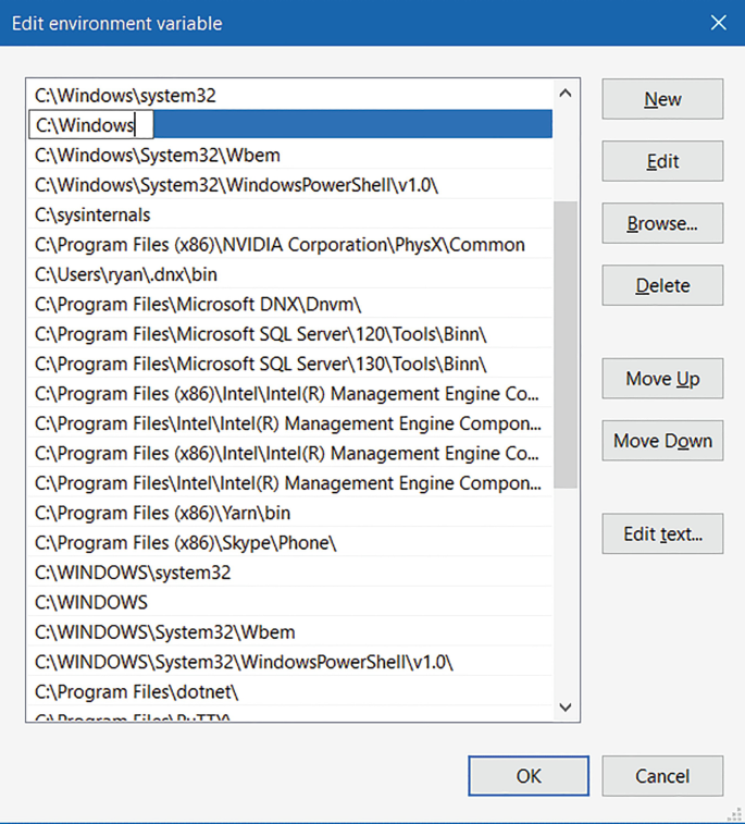
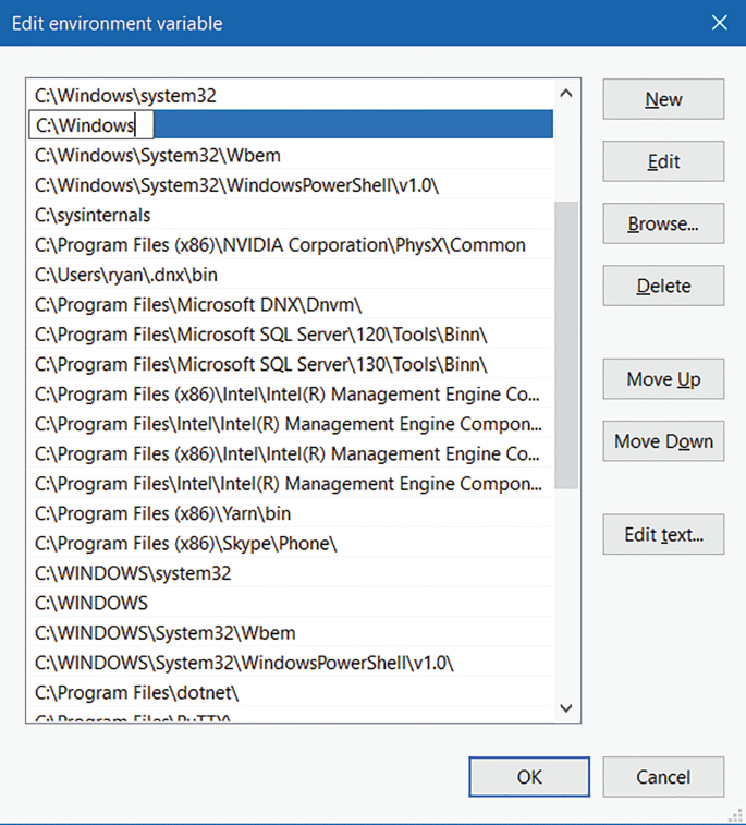
• 4. The “Edit environment variable” UI will appear. Here, you can click “New” and type in the new path you want to add. From this screen you can also edit or reorder them.

  

• 5. Dismiss all the dialogs by selecting “OK”. Your changes are saved! You will probably need to restart apps for them to recognize the change. Restarting your computer would ensure that all apps are run with the PATH change. Open the Start Search, type in “env” and choose “Edit the system environment variables”:

In Linux and MacOS: Depending on the shell you use, you can add a new directory to the PATH environment variable. If you use Bash, you can add the following line in the “~/.profile” or “~/.bashrc” files.

export PATH="$PATH:/ful_path_to_the_folder"

1.1.2 Tensorflow and Keras Installation

Below are the instructions to be able to use tensorflow and keras in R:

• 1. (Only for Windows users) Install Rtools.

  • You can download the official installer from the Rtools official site, then executing the installer is a matter of a few clicks. Once installed, add the path where Rtools was installed to the PATH environment variable. See the Change PATH environment variable section.

• 2. Install the latest version of Python.

  • From the Python official site you can download the official installer for all the most popular operating systems. Once installed, add the path where Python was installed to the PATH environment variable. See the Change PATH environment variable section.

• 3. Install tensorflow and keras Python’s libraries.

  • Open a new terminal (CMD in Windows) and run the following command:

  • python -m install tensorflow keras

• 4. Install the latest tensorflow and keras libraries for R.

  • Open R from the terminal or a new session in RStudio, and run the following commands:

  • if (!require("devtools")) { install.packages("devtools") } install_github("rstudio/tensorflow") install_github("rstudio/keras"),

  • These commands will install tensorflow, keras and all their dependencies.

• 5. Set RETICULATE_PYTHON.

  • To specify to R what Python version it must use, a new environment variable called RETICULATE_PYTHON must be set, that will contain the full path to the Python binary that is usually the path where Python was installed, followed by “/bin/python3.x.x”. The numbers in the xs depends on the version you install. This can be done with the following command.

  • cat( "/full_path/to/python3.x.x", file = "~/.Renviron", append = TRUE ),

  • This command will create a file called. Renviron with this variable that will be loaded each time a new R session starts.

• 6. Restart R.

  • Enjoy of tensorflow and keras in R.

  • This section explains how to install and configure tensorflow and keras globally. This will work for all your projects. If you want to install tensorflow with anaconda or use it in different virtual environments, you may see the reticulate library.

References

Meuwissen THE, Hayes BJ, Goddard ME (2001) Prediction of total genetic value using genome-wide dense marker maps. Genetics 157:1819–1829
Vivek BS et al (2017) Use of genomic estimated breeding values results in rapid genetic gains for drought tolerance in maize. Plant Genome 10:1–8
Crossa J, Pérez-Rodríguez P, Cuevas J, Montesinos-López OA, Jarquín D, de Los Campos G, Burgueño J, González-Camacho JM, Pérez-Elizalde S, Beyene Y, Dreisigacker S, Singh R, Zhang X, Gowda M, Roorkiwal M, Rutkoski J, Varshney RK (2017) Genomic selection in plant breeding: methods, models, and perspectives. Trends Plant Sci 22(11):961–975
Montesinos-López OA, Montesinos-López JC, Singh P, Lozano-Ramirez N, Barrón-López A, Montesinos-López A, Crossa J (2020) A multivariate Poisson deep learning model for genomic prediction of count. G3 (Bethesda) 10(11):4177–4190
Montesinos-López OA, Montesinos-López A, Pérez-Rodríguez P, Barrón-López JA, Martini JWR, Fajardo-Flores SB, Gaytan-Lugo LS, Santana-Mancilla PC, Crossa J (2021) A review of deep learning applications for genomic selection. BMC Genomics 22:19. https://doi.org/10.1186/s12864-020-07319-x
Montesinos-López OA, Martín-Vallejo J, Crossa J, Gianola D, Hernández-Suárez CM, Montesinos-López A, Juliana P, Singh R (2019a) New deep learning genomic prediction model for multi-traits with mixed binary, ordinal, and continuous phenotypes. G3 (Bethesda) 9(5):1545–1556
Montesinos-López OA, Montesinos-López A, Crossa J, Cuevas J, Montesinos-López JC, Salas-Gutiérrez Z, Philomin J, Singh R (2019b) A Bayesian genomic multi-output regressor stacking model for predicting multi-trait multi-environment plant breeding data. G3 (Bethesda) 9(10):3381–3393
Jia Y, Jannink J-L (2012) Multiple-trait genomic selection methods increase genetic value prediction accuracy. Genetics 192(4):1513–1522. https://doi.org/10.1534/genetics.112.144246
Jiang J, Zhang Q, Ma L, Li J, Wang Z, Liu JF (2015) Joint prediction of multiple quantitative traits using a Bayesian multivariate antedependence model. Heredity 115(1):29–36
He D, Kuhn D, Parida L (2016) Novel applications of multitask learning and multiple output regression to multiple genetic trait prediction. Bioinformatics 32(12):i37–i43. https://doi.org/10.1093/bioinformatics/btw249
Schulthess AW, Zhao Y, Longin CFH, Reif JC (2017) Advantages and limitations of multiple-trait genomic prediction for fusarium head blight severity in hybrid wheat (Triticum aestivum L.). Theor Appl Genet 131(3):685–701. https://doi.org/10.1007/s00122-017-3029-7
Calus MP, Veerkamp RF (2011) Accuracy of multi-trait genomic selection using different methods. Genet Sel Evol 43(1):26. https://doi.org/10.1186/1297-9686-43-26
Montesinos-López OA, Montesinos-López A, Crossa J, Toledo F, Pérez-Hernández O, Eskridge KM, Rutkoski J (2016) A genomic Bayesian multi-trait and multi-environment model. G3 (Bethesda) 6(9):2725–2744
Montesinos-López A, Montesinos-López OA, Gianola D, Crossa J, Hernández-Suárez CM (2018a) Multivariate Bayesian analysis of on-farm trials with multiple-trait and multiple-environment data. Agron J:2658–2669. https://doi.org/10.2134/agronj2018.06.0362
Montesinos-López OA, Montesinos-López A, Gianola D, Crossa J, Hernández-Suárez CM (2018b) Multi-trait, multi-environment deep learning modeling for genomic-enabled prediction of plant. G3: genes, genomes. Genetics 8(12):3829–3840
Huang M, Chen L, Chen Z (2015) Diallel analysis of combining ability and heterosis for yield and yield components in rice by using positive loci. Euphytica 205(1):37–50
Montesinos-López A, Montesinos-López OA, Gianola D, Crossa J, Hernández-Suárez CM (2018c) Multi-environment genomic prediction of plant traits using deep learners with a dense architecture. G3 (Bethesda) 8(12):3813–3828. https://doi.org/10.1534/g3.118.200740
Allaire JJ, Chollet F (2019). Keras: R Interface to Keras. https://CRAN.R-project.org/package=keras
VanRaden PM (2008) Efficient methods to compute genomic predictions. J Dairy Sci 91:4414–4423
Chollet F, Allaire JJ (2017) Deep learning with R. In: Manning Early Access Program (MEA) first edition. Manning Publications, Shelter Island, New York
Patterson J, Gibson A (2017) Deep learning a Practitioner’s approach. O’Reilly Media, Sebastopol, California
Cybenko G (1989) Approximations by superpositions of sigmoidal functions. Math Control Signal Syst 2:303–314
R Core Team. (2019). R: a language and environment for statistical computing. R Foundation for Statistical Computing. Vienna. Austria. ISBN 3–900051–07-0. http://www.R-project.org/
González-Camacho JM, Ornella L, Pérez-Rodríguez P, Gianola D, Dreisigacker S, Crossa J (2018) Applications of machine learning methods to genomic selection in breeding wheat for rust resistance. Plant Genome 11(2):1–15. https://doi.org/10.3835/plantgenome2017.11.0104
Gelman A, Rubin D (1992) Inference from iterative simulation using multiple sequences. Stat Sci 7(4):457–511
Allaire JJ (2018) Tfruns: training run tools for “Tensorflow”. https://CRAN.R-project.org/package=tfruns
Author information
Authors and Affiliations
Corresponding authors
Editor information
Editors and Affiliations