
Abstract
The paper describes an eye-tracking study focused on evaluation of 2D and 3D visualization techniques in cartography. Three-dimensional visualization is used by an increasing number of visualization applications and systems. However, there is still too little known about when it is appropriate to do so, and how 3D can be used in visualization most efficiently. The case study contained maps of the cities, where 3D effect was illustrated by 3D buildings. Eye-tracking study was performed to compare user perception of these two types of visualization in maps of the cities. SMI RED 250 eye-tracker with sample frequency of 120 Hz was used in the study. Set of static image stimuli was used for the experiment. Study was performed in within-subject design. For the avoidance of the learning effect, stimuli were modified a bit. Point symbols are placed in different locations, but their number is the same for each pair of stimuli. For evaluation of results, statistical analyses of selected eye-tracking metrics were used, as well as the visual analytics of eye-tracking data. Eye-tracking experiment was enhanced with a questionnaire, examining the respondent’s subjective opinions about each visualization technique. It was found, that 3D effect in city maps without tilt has no influence on map reading. Searching for point symbols was not different between maps with and without 3D effect.
Keywords
Introduction
There are several perspectives on the term “3D” in cartography. Kraak (1988) in one of the first articles focused on 3D maps states that image will be considered 3D if it contains those stimuli or depth cues which make it being perceived as 3D.
Wood et al. (2005) described the role of three dimensionality used in both process of visualization and representation of 3D objects and space. To clarify the term “3D”, they considered the model of a general visualization pipeline. According to Upson et al. (1989) and Haber and McNabb (1990) it is possible to distinguish five levels of dimensionality, which correspond to the various stages within a visualization process (data management, data assembly, visual mapping, rendering, display). Wood et al. (2005) associates the term 3D with the phase of “visual representations of data”, but it can also be part of the outputs from all other stages of the process.
Non-photorealistic Models of the Cities
According to Cartwright et al. (2007), two basic concepts of 3D cartography exist—photorealistic and non-photorealistic. Durand (2002) emphasizes that non-photorealistic visualization provides “extensive control over expressivity, clarity and aesthetics”, but Jedlicka et al. (2013) mentions also the limits (generalisation, simplification, non-perspective projections, distortions etc.)
This general fact could be applied also for the visualization of cities. Photorealistic visualization of cities became popular due to the ubiquity of Google Earth and similar applications, where models of large areas are created with automatic or semi-automatic acquisition method. Models are created in high detail, and aerial photo is used as a base map. Because of the lack of the clarity, it is difficult to use photorealistic visualization as the map of larger areas. Non-photorealistic models influence the map complexity too, but not so significantly.
Generally characteristics of non-photorealistic rendering techniques include the ability to sketch geometric objects and scenes, to reduce visual complexity of images, as well as to imitate and extend classical depiction techniques known from scientific and cartographic illustrations (Döllner and Buchholz 2005). Standardization of 3D maps was discussed in Herman and Reznik (2013).
Modern internet map portals use non-photorealistic 3D models in different levels of abstraction as an enhancement of the map, especially in large cities. Maps used as stimuli in the experiment are described in chapter “Stimuli” in more detail.
Evaluation of 3D Maps
Three dimensional non-photorealistic 3D visualization is used by an increasing number of applications. However, there is a still little known how 3D can be used in visualization most efficiently. As Konečný et al. (2011) highlights, the creation of the usability tests for different types of maps and visualizations is quite a challenge.
There exist few studies, focused on evaluation of 3D in maps. Most of them use the questionnaire as the main investigation method. Savage et al. (2004) and Petrovic and Masera (2006) analysed user’s preferences on 2D and 3D maps. Schobesberger and Patterson (2008) investigate differences between 2D and 3D map of the Zion National Park in Utah. Haeberling (2004) evaluated design variables for 3D maps.
In few studies, eye-tracking was used for the evaluation of 3D maps. Fuhrmann et al. (2009) analysed differences between perception of 2D map and its holographic equivalent. Irvankoski et al. (2012) investigates visualization of elevation information on maps. Interaction with a 3D geo-browser under time pressure was evaluated by Wilkening and Fabrikant (2013). Possibilities of eye-tracking evaluation in cartography were discussed in Popelka et al. (2012) and Popelka and Voženílek (2012).
Different perception of 2D and 3D terrain maps was investigated in Popelka and Brychtová (2013). In this study, two eye-tracking tests were used for observing the user perception of the pair of maps representing the terrain. On one map, the terrain was represented by contour lines. Second map contained the perspective view of the same data as the first map.
The purpose of the paper is to analyse the user perception of two types of 3D visualization in maps of the cities.
Case Study
Equipment
For the case study, an eye-tracking device was used. As Ooms et al. (2014) states, eye-tracking is a direct method to study users’ cognitive processes. Eye-tracker is situated in the special room—eye-tracking laboratory. Windows are covered with non transparent foil, to unify the lighting conditions.
SMI RED 250 eye-tracker was used within the study. This device is capable of recording eye-movements with the frequency of 120 Hz. Eye positions are recorded every 8 ms. Eye-tracker is supplemented by web camera, which records participant during the experiment. This video helps to reveal the cause of missing data, respondents’ reactions to the stimuli and their comments to the particular maps.
For data visualization and analyses, three different applications were used. First one is SMI BeGaze, which is software developed by the manufacturer of the device. Open source software OGAMA and CommonGIS developed at Fraunhofer Institute in Germany were used for visual analytics of eye-tracking data.
Participants
Total of 40 participants (24 females, 16 males) attended the eye-tracking experiment. Most of them were representatives of academic staff and students. Respondents were originated from different fields. Some of them were cartographers, some of them were not. Majority of participants were 20–25 years old. Participants were not paid for the testing.
Before the experiment, respondents filled out the short questionnaire with personal information. Apart from elementary information, like age or sex, they had to answer the question, how often are they using the internet map portals like Google Maps or OpenStreetMap. Most of the participants use the web map portals every day.
Experiment Design
At the beginning of the experiment, respondents fill out a short questionnaire. Then, the 9-point calibration was performed. Eye-movement recordings with deviation smaller than 1° were included in the experiment.
After the calibration, welcome screen with instructions was displayed. The instructions included also the sample question. Respondents’ task was to find out one particular point symbol in the map as fast as possible and mark it with the mouse click.
Study was performed in within-subject design. The experiment contained 18 static stimuli with 2D and 3D maps of cities. The stimuli with maps were presented in random order. To unite the starting point of the eye-movement trajectories, the fixation cross was displayed for 500 ms before the stimulus. Respondents had maximum time of 30 s to find the target, but for the most of the tasks, the time was fully sufficient.
Stimuli
The experiment contained screenshots of different internet map portals. These maps were complemented with point symbols. Two types of maps were used—the first one was standard map with buildings represented by polygons, second contained 3D (2,5 D) visualization of buildings.
Maps from three different sources were used. The first one is well-known Google map (stimuli 1–5). In bigger cities, the Google map in zoom 17 and higher contains 3D representation of block of buildings. These screenshots were compared with 2D maps, which were captured in the different part of the city (where 3D coverage was not used) or with the use of merging and scaling down of the map of the same area in zoom 16. The maps were styled (with the use of Gmaps wizard), because the original map available at maps.google.com contains a large amount of symbols and labels. For the purpose of the experiment, the fictitiously placed point symbols (designed according to the original ones from Google Maps) were used. For each pair, the same number and set of symbols was used.
Second type of maps contained maps from OpenStreetMap.org (stimuli 6–8). In the default version, there exists no option to display 3D block of buildings. However, thanks to the free availability of OSM data, there exist some possibilities, how to display 3D content. Well-known is project osmbuildings.org, which is an additional layer to existing web maps. It is currently working with LeafletJS and OpenLayers.
Last stimulus (map 9) also uses OpenStreetMap data through project F4Map. This project is only in beta version, but it automatically creates the 3D variant of cities all over the world. The map is enhanced by ground elevation, animated water, dynamic shadows, urban and natural details. It is possible to switch between 2D and 3D version of the map, but also to change the camera angle and rotation.
The example of each type of stimuli (Google Maps, OSMbuildings and F4map) is in the Fig. 1.

The pair of the stimuli. 2D (left) and 3D (right), where the buildings are represented with 3D blocks. Up: Google Maps (source: http://maps.google.com), Middle: OSMbuildings (source: http://osmbuildings.org), Bottom: F4map (source: http://map.f4-group.com)
Results
Analysis of Questionnaire
Part of the experiment was the questionnaire, focused on participants’ personal opinion about presented maps. The questionnaire was presented after all stimuli, and it contained only two questions. First one concerned the suitability of the map. Respondents were asked to answer, which variant of the map was more suitable for finding the answer. Second question was focused on the aesthetic factor—which variant did they like more. In both questions, three options were available—“2D”; “3D” and “Depends on the specific map”.
Participants found 2D map more suitable for answering the question (finding the point symbol in the map) than 3D map. Majority of them (24 from 40) preferred 2D variant of the map. Relatively high number of respondents (13 from 40) chose answer “Depends on the specific map”.
Participants were also asked, which type of map like they more. The distribution of the preferences between 2D and 3D maps was almost balanced (19 for 2D vs. 13 for 3D).
Fixation Detection
One of the most important issues in eye-tracking data analysis is event detection of recorded data. For almost all analyses, the fixations and saccades are needed. Eye-tracking data were recorded with sample frequency of 120 Hz, so the dispersion algorithm (I-DT), which is more appropriate for the low-frequency data, was used.
IDT takes into account the close spatial proximity of the eye position points in the eye movement trace (Salvucci and Goldberg 2000). The algorithm defines a temporal window which moves one point at a time, and the spatial dispersion created by the points within this window is compared against the threshold. If such dispersion is below the threshold, the points within the temporal window are classified as a part of fixation; otherwise, the window is moved by one sample, and the first sample of the previous window is classified as a saccade (Komogortsev and Khan 2009).
The threshold values were set to 80 ms (duration) and 50 px (dispersion). These values were selected based on the author’s unpublished study, which compares four settings, used in cartographic papers and identified the thresholds, which fits to the recorded raw data.
For data analysis, open-source software OGAMA was also used. Most important parameters are “Maximum distance” and “Minimum number of samples”, which corresponds to dispersion and duration in BeGaze. For optimizing the event detection parameters in OGAMA, the image of scanpath from BeGaze was used in OGAMA instead of SlideResource image. The fixations in OGAMA were plotted over the image of the BeGaze fixations. Event detection parameters in OGAMA were changed until the scanpath was very similar to the scanpath from BeGaze.
Statistical Analysis
For statistical analysis of eye-movement data, several eye-tracking metrics were calculated. For all metrics, median values for 40 respondents were calculated. Median was used instead of mean because the data had not normal distribution and median also filter out the extreme values. Data was analysed with the use of the Wilcoxon rank sum test and statistically significant difference between 2D and 3D maps was observed on the significance level α = 0.05 in all cases.
Analysed metrics were Time to Answer (click), Fixation Count, Fixation Duration Median and Scanpath Length.
In case of Time to Answer metric (Fig. 2, left), highest difference between 2D and 3D variant was observed for map 9. This result was expected, because the 3D map no. 9 is tilted and orientation in this map is harder. Second highest value of Time to Answer was recorded in case of 3D variant of map 5. This map, which displays the downtown of New York with many 3D skyscrapers, is the most complex one from the set of “Google maps (map 1–5)”. It is surprising that the difference between 2D and 3D variant is so small in this case.

Graph of median time to answer (left) and scanpath length (right) values for each map in the experiment
Value of Time to Answer is interlinked with the Fixation Count metric (see Table 1), where statistically significant difference was observed for 7 from 9 maps. In contrast to Fixation Count, statistically significant difference for Fixation Duration Median was observed only in three cases (Map 5, 7 and 9).
According to Goldberg et al. (2002), a longer scanpath indicates less efficient searching. Statistically significant difference was found in 5 cases from 9 (Fig. 2, right). For maps 1 and 7, higher median scanpath length was recorded for 2D variant. For maps 3, 6 and 9, higher values were recorded for 3D variant. This fact suggests that the scanpath length was dependent on other variable than 2D or 3D visualization method.
Apart from the analyses for particular maps; also the whole dataset for all maps was analysed (see Table 2). It was found that results for map 9 influenced all results. If the map 9 was included in the dataset, statistically significant differences were found for Time to Answer and Fixation Duration Median. The values were higher for the 3D map. When the map 9 data were omitted, with the Wilcoxon rank sum test on the significance level α = 0.05, no differences between 2D and 3D variant were found for any of the metrics.
Statistical analysis showed that there are statistically significant differences in eye-tracking metrics between 2D and 3D variant of a particular map, but the results did not indicate that one of the variants is better than the other. Within the analysis of the entire dataset as a sum of all maps, no statistically significant differences were found for any of the studied eye-tracking metric.
Visual Analytics of Data
Visual analytics, the science of analytical reasoning facilitated by interactive visual interfaces is an important tool for investigation of a large amount of data. For the visual analytics of recorded eye-tracking data, software CommonGIS developed at the Fraunhofer Institute IAIS was used. For data conversion from BeGaze software to CommonGIS environment, the conversion tool created by Kristien Ooms was used. Fixations from BeGaze software were transformed into the trajectories, which are represented as lines in CommonGIS.
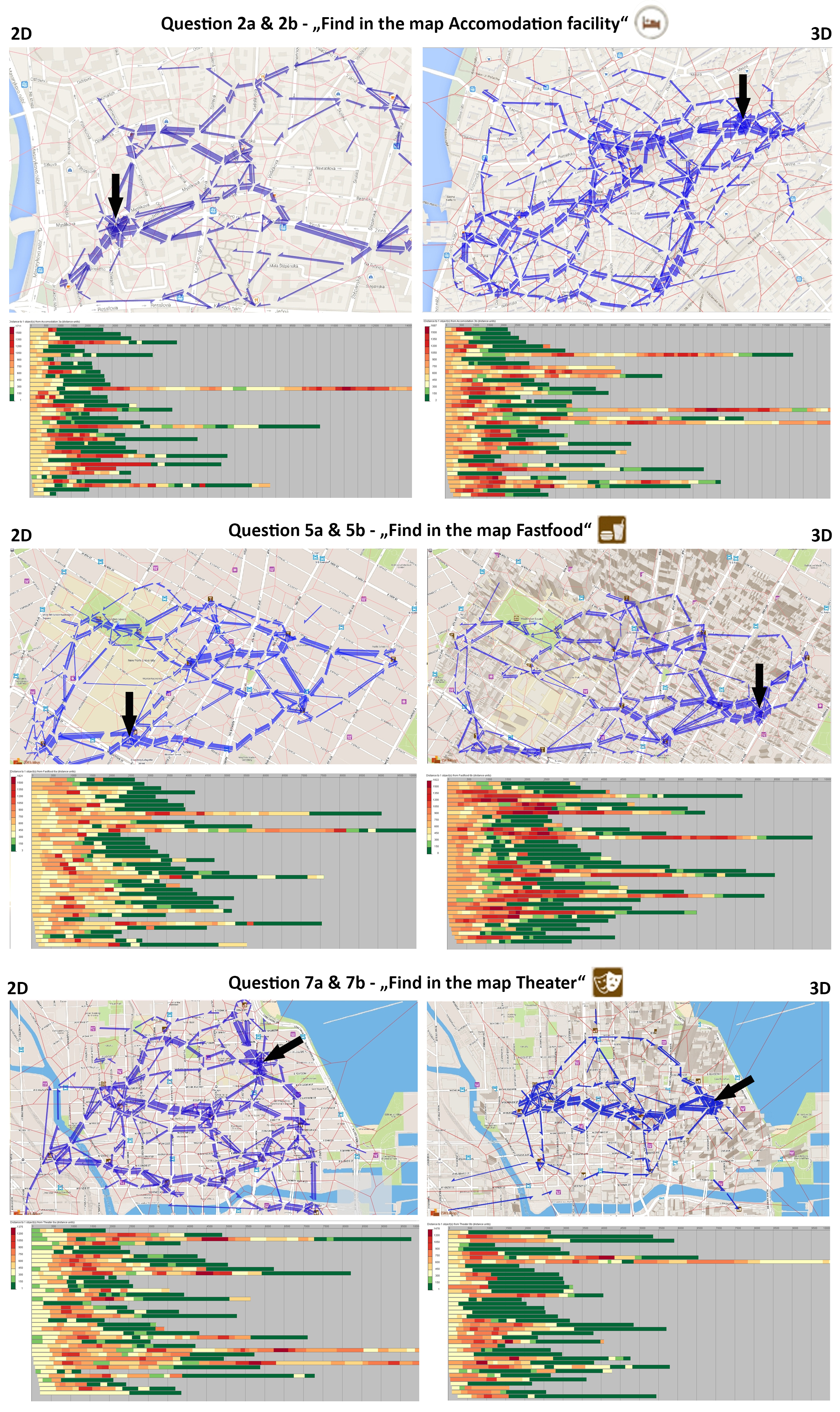
For data analyses, two methods introduced by Andrienko et al. (2012) were used. First method, Flow Map, represent results of discrete spatial and spatio-temporal aggregation of trajectories. Arrows represent multiple movement of gaze from one location to another. The thickness of arrows is derived from variable Number of moves between defined voronoi polygons. Only arrows representing more than three moves are displayed.
Second used method is Temporal View of Trajectories. The horizontal dimension of the graph represents time, and the colour of the lines displays the distance between current gaze position and the target in pixels.
In Fig. 3, three map pairs are shown. First image from the top shows the situation, when more of cumulative gaze trajectories were observed in case of 3D variant of the map (right part of the image). The Temporal View shows that respondents spent more time in the map until they found the target. In the middle of the Fig. 3, the gaze trajectories are similar for both variants (2D and 3D). Image at the bottom of shows the situation, where more trajectories were observed in the 2D map.

Visual analytics of selected tasks in CommonGIS. Black arrows point to the location of correct answer. 2D variant is on the left, 3D on the right. Figure in full resolution is available at www.eyetracking.upol.cz/Research_images/Cities.jpg
Conclusion
Locations of the targets in the experiment tasks were placed in similar distance from the centre of the image (where respondents gaze starts) for both variants of the map. Nevertheless in some cases, answers were faster in 2D map, in some cases in the 3D one. Data from the short questionnaire after the experiments shows that respondents consider the 2D variant more suitable for answering the question. No significant differences between 2D and 3D maps were found for four metrics (Time to Answer, Fixation Count, Fixation Duration Median and Scanpath Length). Respondents also did not clearly incline to the one of variants from the aesthetics point of view.
Point symbol search was more difficult on the map where 3D effect was created with use of map tilt (map no. 9). For this map, statistically significant differences were observed for all recorded eye-tracking metrics. This type of maps should not be used very often, because users have problems with orientation in this map.
On the other hand, results for all other stimuli (maps no 1–8) indicate that in situations when it is reasonable and desirable, the 3D map of the city could be used instead of the standard two-dimensional. In the three-dimensional map, more information is contained and the 3D representation did not influence the reading of the map and its comprehensibility.
References
Andrienko G, Andrienko N, Burch M, Weiskopf D (2012) Visual analytics methodology for eye movement studies. IEEE Trans Vis Comput Graph 18(12):2889–2898
Cartwright W, Peterson MP, Gartner G (2007) Multimedia cartography. Springer, Heidelberg
Döllner J, Buchholz H (2005) Non-photorealism in 3D geovirtual environments. In: Proceedings of AutoCarto, ACSM, Las Vegas, pp 1–14
Durand F (2002) An invitation to discuss computer depiction. In: Symposium on non-photorealistic animation and rendering (NPAR)
Fuhrmann S, Komogortsev O, Tamir D (2009) Investigating hologram-based route planning. Trans GIS 2009:177–196
Goldberg JH, Stimson MJ, Lewenstein M, Scott N, Wichansky AM (2002) Eye tracking in web search tasks: design implications. In: Proceedings of the eye tracking research and applications symposium, New Orleans, 25–27 March, pp 51–58
Haber RB, McNabb DA (1990) Visualization idioms: a conceptual model for scientific visualization systems. In: Nielson G, Shriver B, Rosenblum L (eds) Visualization in scientific computing. IEEE Computer Society Press, Los Alamitos, pp 74–93
Haeberling C (2004) Topografische 3D-Karten ñ Thesen für kartografische Ge-staltungsgrundsaetze. Dissertation, Institut für Kartographie der ETH Zuerich, Zuerich
Herman L, Reznik T (2013) Web 3D visualization of noise mapping for extended INSPIRE buildings model. In: Hrebicek J et al (eds) ISESS 2013, IFIP AICT 413, pp 414–424
Irvankoski K, Torniainen J, Krause CM (2012) Visualisation of elevation information on maps: an eye movement study. In: Conference proceedings, The Scandinavian Workshop on Applied Eye Tracking (SWAET), Karolinska Instituet, Stockholm, 56 p
Jedlicka K, Cerba O, Hajek P (2013) Creation of information-rich 3D model in geographic information system – case study at the Castle Kozel. In: Conference proceedings, informatics, geoinformatics and remote sensing, vol I. STEF92 Technology Ltd., Sofia, pp 685–692
Komogortsev O, Khan J (2009) Predictive compression for real time multimedia communication using eye movement analysis. ACM Transactions on Multimedia Computing, Communications and Applications 6
Konečný M, Kubíček P, Stachoň Z, Šašinka C (2011) The usability of selected base maps for crises management – users’ perspectives. Appl Geomatics 3(4):189–198
Kraak MJ (1988) Computer-assisted cartographic three-dimensional imaging techniques. In: Raper J (ed) Three dimensional applications in geographical information systems. Taylor & Francis, London, pp 99–114
Ooms K, De Maeyer P, Fack B (2014) Study of the attentive behavior of novice and expert map users using eye tracking. Cartogr Geogr Inf Sci 41(1):37–54
Petrovic D, Masera P (2006) Analysis of user’s response on 3D cartographic presentations. In: Proceedings of 5th ICA mountain cartography workshop, Bohinj
Popelka S, Brychtová A (2013) Eye-tracking study on different perception of 2D and 3D terrain visualisation. Cartogr J 50(3):240–246s. ISSN: 1743–2774 (Maney Publishing)
Popelka S, Voženílek V (2012) Specifying of requirements for spatio-temporal data in map by eye-tracking and space-time-cube. In: Proceedings of international conference on graphic and image processing, Singapore, 5 p
Popelka S, Brychtová A, Voženílek V (2012) Eye-tracking a jeho využití při hodnocení map. Geografický časopis Geografický ústav SAV, pp 71–87
Salvucci DD, Goldberg JH (2000) Identifying fixations and saccades in eye tracking protocols. Eye tracking research and applications symposium. ACM, New York
Savage DM, Wiebe EN, Devine HA (2004) Performance of 2D versus 3D topographic representations for different task types. Proc Hum Factors Ergon Soc Annu Meet 48(16):1793–1797
Schobesberger D, Patterson T (2008) Exploring of effectiveness of 2D vs. 3D trail-head maps. In: Proceedings of 6th ICA mountain cartography workshop, Lenk im Simmental
Upson C, Faulhaber T, Kamins D, Schlegel D, Laidlaw D, Vroom J, Gurwitz R, van Dam A (1989) The application visualization system: a computational environment for scientific visualization. IEEE Comput Graph Appl 9(4):30–42
Wilkening J, Fabrikant SI (2013) How users interact with a 3D geo-browser under time pressure. Cartogr Geogr Inf Sci 40(1):40–52
Wood J, Kirschenbauer S, Döllner J, Lopes A, Bodum L (2005) Using 3D in visualization. In: Dykes J, MacEachren AM, Kraak M-J (eds) Exploring geovisualization. Pergamon, Oxford, pp 295–312
Author information
Authors and Affiliations
Corresponding author
Editor information
Editors and Affiliations
Rights and permissions
Copyright information
© 2015 Springer International Publishing Switzerland
About this chapter
Cite this chapter
Popelka, S., Doležalová, J. (2015). Non-photorealistic 3D Visualization in City Maps: An Eye-Tracking Study. In: Brus, J., Vondrakova, A., Vozenilek, V. (eds) Modern Trends in Cartography. Lecture Notes in Geoinformation and Cartography. Springer, Cham. https://doi.org/10.1007/978-3-319-07926-4_27
Download citation
DOI: https://doi.org/10.1007/978-3-319-07926-4_27
Published:
Publisher Name: Springer, Cham
Print ISBN: 978-3-319-07925-7
Online ISBN: 978-3-319-07926-4
eBook Packages: Earth and Environmental ScienceEarth and Environmental Science (R0)