
Abstract
Digital multiple notch filters are used in a variety of applications to remove or suppress multiple sinusoidal or narrow-band interference in digital signals. In this paper, we propose an all-pass filter-based design framework for infinite impulse response (IIR) multiple notch filters. Our approach aims to overcome the limitations of former techniques through greater design capacity and performance. The proposed framework has versatility and enables the tailored use of design constraints thus providing a family of possible multiple notch filter design methods. The design performance and practicality of the proposed framework are verified empirically by a series of experimental results and different applications.
1 Introduction
Digital notch filters are used to eliminate sinusoidal or narrow-band interference in digital signals while preserving the other frequency components intact [1-4]. They have been widely applied in a variety of disciplines ranging from audio signal processing to biomedical engineering [5-19]. Recently, there has been interest in designing multiple-frequency notch filters that aim to suppress two or more frequencies of an input signal [20-25]. Two types, finite-impulse response (FIR) and infinite-impulse response (IIR), exist. As typical, the former exhibits advantages of linear phase and stability while the latter has advantages of narrower stop-band and higher quality factor for the same filter order of more significance to notch filter design [26-34].
Several approaches exist to design IIR multiple notch filters [1-3,21-23,35-40]. The cascading method is a popular direct design technique that realizes a multiple notch filter by cascading several well-designed second-order IIR single-notch filters [36]. The resulting system is characterized by a canonical structure for software and hardware realization. The main drawback is that it is restricted to few notch frequencies and very narrow bandwidths otherwise leading to non-unity pass-band gains [37].
The optimal design method requires computations for pole placement that results in a better frequency characteristic [2,3,37,38], but highly complex search-based or iterative algorithms are required even for a notch filter with two frequencies [2,38]. For a greater number of notch frequencies, a two-stage approach has been proposed to generate a stable optimal multiple notch filter, but the design procedure involves quadratic programming via an iterative scheme [3].
The all-pass filter-based method presented by S-C. Pei and C-C. Tseng transforms the specifications of a multiple notch filter to those of an equivalent all-pass filter. A linear design equation is constructed to determine the all-pass filter coefficients which are used to characterize the desired multiple notch filters [1,41]. An improved method was proposed to design a notch filter with only two frequencies [42]. One advantage is that all-pass filter-based methods have normalized analytical forms with no iterative calculations.
The practical success of all-pass filter-based methods is a result of three assumptions: i) the magnitude responses are symmetric about notch frequencies, ii) the neglected right-hand cutoff frequencies do not produce design errors, and iii) the constructed linear equation has an accurate solution. However, these constraints can also lead to the following challenges [42]. The symmetric magnitude responses are too prohibitive for applications. The information of the all-pass filter is not fully utilized. And, the linear equation is potentially ill-conditioned due to tangent operations.
Thus in this work, we present a generalized design framework for IIR multiple notch filters whereby we aim to: a) deduce an improved design process of the all-pass filter-based method, b) maximize the availability of phase information of all-pass filter, and c) introduce selection mechanisms and weighting strategies to enable the unified representation of a family of all-pass filter-based methods. We also apply the framework to typical multiple notch filter applications to empirically test performance.
In the next section, an improved all-pass filter-based approach is explored for multiple notch filters. Section 2 proposes a generalized framework with selection mechanisms and weighting strategies. Section 2 verifies the effectiveness and practicality of our framework through experimental results. Final conclusions are drawn in Section 2.
2 Improved multiple notch filter design
Suppose s[n] is a desired information-bearing signal corrupted by N sinusoidal interference components whose frequencies are ω N1,ω N2,⋯,ω NN . The overall corrupted signal can be expressed as [1,2]:
where A i and ϕ i represent the magnitude and initial phase of the ith sinusoidal component.
In order to extract s[n] from x[n] with limited distortion, the design specification of an ideal digital multiple notch filter is given by [2]:
where i=1,2,⋯,N. Without loss of generality, we assume ω N1<ω N2<⋯<ω NN . In practice, zero bandwidths can not be realized [22]. Hence, the frequency response of an actual notch filter is the approximation to that of the ideal one.
2.1 All-pass filter-based design process
In this section, we reformulate the all-pass filter-based design process of multiple notch filters. Suppose that the notch frequencies ω N1,ω N2,⋯,ω NN correspond to notch bandwidths B N1,B N2,⋯,B NN , respectively. The system function of the notch filter is expressed as follows [1,3]:
where A(z) is an 2N-order all-pass filter.
The frequency response of the notch filter is given by:
where ω∈(−π,π]. The all-pass filter has magnitude response |A(e jω)|=1 and phase response θ A (ω)=∠ A(e jω) that is monotonically decreasing [43]. For an 8-order all-pass filter (N=4), its magnitude and phase responses are shown in Figure 1. Thus, A(e jω) can be uniquely characterized by θ A (ω):

Frequency responses of an 8-order ( N =4) all-pass filter. (A) Amplitude response. B Phase response.
Therefore, θ A (ω) must be carefully selected such that H(e jω) fulfills the design specifications (notch frequencies and bandwidths) of the notch filter.
Generally, a 2N-order all-pass filter is expressed as:
where real coefficients a k ∈ℝ (k=1,2,⋯,2N) in both the numerator and denominator polynomials [1,3]. Given the formulation in Equation 4, determining appropriate values of a 1,a 2,⋯,a 2N represents the core problem of all-pass filter-based multiple notch filter design.
To determine a 1,a 2,⋯,a 2N , we relate them to the multiple notch filter design specifications as follows. Rearranging Equation 6 gives:
Next, substituting z=e jω and Equation 5 into the left-hand side of Equation 7 gives:
Correspondingly, the right-hand of Equation 7 becomes:
Therefore, Equation 10 can also be expressed as:
Then, we obtain Equation 12 from Equation 11:
By equating the real and imaginary parts of Equation 12 and applying triangular identities: cos(α−β)= cosα cosβ+ sinα sinβ and sin(α−β)= sinα cosβ− cosα sinβ, we deduce:
and
Finally, adding both sides of Equations 13 and 14 together gives:
Thus to solve for a 1,a 2,⋯,a 2N , at least 2N distinct pairs (ω,θ A (ω)) must be known to provide at least 2N equations to solve 2N unknowns.
Suppose M-pairs (ω,θ A (ω)) denoted {(ω m ,θ A (ω m ))|m=1,2,⋯,M} are known. Then, a linear equation containing M identities with 2N variables a 1,a 2,⋯,a 2N can be constructed from Equation 15 and represented by:
where Q=[q mk ] is a M×2N matrix, a=[a 1,a 2,⋯,a 2N ]T is a 2N×1 vector, and p=[p 1,p 2,⋯,p M ]T is an M×1 vector such that:
and
It is well known that a unique solution to Equation 16 exists if M=2N and Q is non-singular. For M>2N, Equation 16 only has a least-square solution [44].
Based on the above discussion, our proposed design process works as follows. Given the N notch frequencies ω N1,ω N2,⋯,ω NN and corresponding bandwidths specifications B N1,B N2,⋯,B NN for the multiple notch filter:
-
1.
Choose the related all-pass filter design constraints {(ω m ,θ A (ω m ))| m=1,2,⋯,M } to construct Equation 16 where M≥2N.
-
2.
Solve the linear equations of Equation 16 to obtain the all-pass filter coefficient vector a=[a 1,a 2,⋯,a 2N ]T.
-
3.
Substitute a 1,a 2,⋯,a 2N into Equation 6 and then Equation 3 to obtain the multiple notch filter system function H(z).
We assert that step 1 will have a significant impact on the quality of the multiple notch filter design. Thus, in the next section, we assess four strategies to select design constraints that we verify and compare empirically in Section 2.
2.2 Constraint selections of notch filter design
For a 2N-order all-pass filter, its phase response θ A (ω) is monotonically decreasing from 0 to −2N π as illustrated in Figure 1. Given the continuity of both ω and θ A (ω), there are an uncountably infinite number of (ω,θ(ω)) pairs that can be selected for notch filter design by Equation 16. However, if we restrict ourselves to those quantities related to the design specifications of the multiple notch filter, we can naturally arrive at 3N pairs that may be used. Specifically, those pairs related to the notch frequencies and left-hand and right-hand 3 dB cut-off frequencies employed [1].
Figure 2 illustrates the relationship between θ A (ω) and |H(e jω)| to ensure that Equation 4 results in a suitable notch filter frequency response that we detail as follows:
-
1.
At notch frequencies, θ A (ω) must be equal to an odd multiple of π to ensure that |H(e jω)|=0. Specifically, we require that θ A (ω Ni )=−(2i−1)π,(i=1,2,⋯,N), to give \(A\left (e^{j\omega _{\textit {Ni}}}\right)= e^{j\theta _{A}(\omega _{\textit {Ni}})}=-1\) resulting in \(|H\left (e^{j\omega _{\textit {Ni}}}\right)|=0\). Therefore, {(ω Ni ,θ A (ω Ni ))| i=1,2,⋯,N } gives \(\phantom {\dot {i}\!}|H(e^{j\omega _{\textit {Ni}}})|=0\) at the N notch frequencies providing a valuable set of filter design constraints.
Figure 2 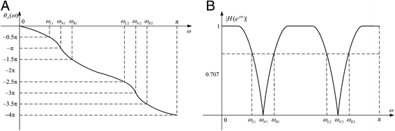
The relations between phase response of all-pass filter and magnitude response of multiple notch filter. (A) Phase response of all-pass filter. (B) Magnitude response of notch filter.
-
2.
Next, at the left-hand 3 dB frequencies, θ A (ω) must appropriately ensure that \(|H\left (e^{j\omega }\right)|=\sqrt {2}/2\). One way to achieve this is to let θ A (ω Li )=−(2i−1)π+π/2,(i=1,2,⋯,N) such that \(A\left (e^{j\omega _{\textit {Li}}}\right)= e^{j\theta _{A}(\omega _{\textit {Li}})}=-j\) resulting in \(|H\left (e^{j\omega _{\textit {Li}}}\right)|=\sqrt {2}/2\). Thus, {(ω Li ,θ A (ω Li ))|i=1,2,⋯,N} gives \(|H\left (e^{j\omega _{\textit {Li}}}\right)|=\sqrt {2}/2\) providing another valuable set of filter design constraints.
-
3.
Similarly, the right-hand 3 dB frequencies with θ A (ω Ri )=−(2i−1)π−π/2,(i=1,2,⋯,N) give \(A\left (e^{j\omega _{\textit {Ri}}}\right)= e^{j\theta _{A}(\omega _{\textit {Ri}})}=j\) resulting in \(|H\left (e^{j\omega _{\textit {Ri}}}\right)|=\sqrt {2}/2\) providing {(ω Ri ,θ A (ω Ri ))|i=1,2,⋯,N} as the third set of filter design constraints.

Those relations are summarized in Table 1. It provides 3N possible (ω,θ A (ω)) pairs for notch filter design. However, given that only 2N are needed to solve Equation 16, four intuitive and effective selection methods from the 3N-pair parameters are possible as highlighted in Table 2.
The reader should note that each selection method from Table 2 provides sufficient information to solve Equation 16 since M≥2N, but they may lead to slightly different results for the same design specifications. We evaluate their design performance in Section 2 but characterize each approach briefly below.
Method I utilizes notch and left-hand cutoff frequencies as filter design constraints, which is suitable for the case of very narrow interference bandwidths and symmetrical magnitude responses about the notch frequencies. Method I is adopted in [1].
Method II, in contrast to method I, utilizes notch and right-hand cutoff frequencies for filter design. Roughly, it has the same applicability and limitations as method I, but the results of method II are slightly different from those of method I.
Method III employs left-hand and right-hand cutoff frequencies as the constraints for filter design. Although it is not limited to very narrow notch bandwidths and symmetrical magnitude responses, it may result in notch frequencies drifting from their desired positions.
Method IV makes use of all available information: notch frequencies and both left-hand and right-hand cutoff frequencies. Thus, it is able to realize a trade-off between notch bandwidths and notch positions effectively enhancing the design performance. The constraint selection method is also adopted by method V in Section 2.
The reader should note that M=2N in methods I, II, and III produce unique solutions. In contrast to method IV, M=3N results in an over-determined equation with a least-square solution. However, we aim to unify both into a generalized design framework that we present next.
3 Multiple notch filter design framework
3.1 Matrix representations of selection methods
The options for constraints of multiple notch filter design discussed in Section 2 can be described collectively via vector-matrix forms. Let N notch frequencies, N left-hand and N right-hand cutoff frequencies be denoted as ω N = [ω N1,ω N2,⋯,ω NN ]T, ω L = [ω L1,ω L2,⋯,ω LN ]T, and ω R = [ω R1,ω R2,⋯,ω RN ]T, respectively. We also denote the N×N zero matrix with 0 and the N×N identity matrix with I. The selected frequencies can be expressed as:
where ω and \(\boldsymbol {\hat \omega }\) are 3N×1 vectors. \({\boldsymbol {\hat \omega }}_{L}\), \({\boldsymbol {\hat \omega }}_{N}\), and \({\boldsymbol {\hat \omega }}_{R}\) are N×1 vectors. S=diag(S L ,S N ,S R ) is a 3N×3N diagonal matrix. S L , S N , and S R are N×N sub-matrices equal to either 0 or I such that S maps the set of all possible frequencies of interest ω to \(\boldsymbol {\hat \omega }\) employed for notch filter design.
From Table 2, it is clear that at least two sub-matrices of S must be set as I. For example, for S L =S N =I and S R =0, \({\boldsymbol {\hat \omega }}_{L}={\boldsymbol {\omega }}_{L}\), \({\boldsymbol {\hat \omega }}_{N}={\boldsymbol {\omega }}_{N}\), and \({\boldsymbol {\hat \omega }}_{R}=\bf {0}\), which corresponds to method I that only makes use of notch and left-hand cut-off frequencies. Table 3 relates the specific sub-matrix values to all selection methods discussed in Section 2.
For convenience, we abbreviate all-pass phases θ A (ω Li ), θ A (ω Ni ), and θ A (ω Ri ) as θ Li , θ Ni , and θ Ri , respectively, for i=1,2,⋯,N. Similarly, we define N×1 vectors θ L =[θ L1,θ L2,⋯,θ LN ]T, θ N = [θ N1,θ N2,⋯,θ NN ]T, and θ R = [θ R1,θ R2,⋯,θ RN ]T which correspond to ω L , ω N , and ω R , respectively. A similar vector-matrix form related to all-pass filter phases is expressed as follows:
where θ and \({\boldsymbol {\hat {\theta }}}\) are 3N×1 vectors; \({\boldsymbol {\hat \theta }}_{L}\), \({\boldsymbol {\hat \theta }}_{N}\), and \({\boldsymbol {\hat \theta }}_{R}\) are N×1 vectors correspond to θ L , θ N , and θ R respectively; S has the same meaning as in Equation 19.
Therefore, four selection methods of (ω,θ A (ω)) in Table 2 can be uniformly represented via Equations 19 and 20 whereby the value of S determines the particular method used for multiple notch filter design.
3.2 Linear equation and least-square solution
If all elements of the selected frequency vector \({\boldsymbol {\hat \omega }}\) and all-pass phase vector \({\boldsymbol {\hat \theta }}\) are substituted into Equations 17 and 18, we obtain the following linear equation from Equation 16:
where \({\boldsymbol {\hat {p}}}_{L}\), \({\boldsymbol {\hat {p}}}_{N}\), and \({\boldsymbol {\hat {p}}}_{R}\) are N×1 vectors; \({\boldsymbol {\hat {Q}}}_{L}\), \({\boldsymbol {\hat {Q}}}_{N}\), and \({\boldsymbol {\hat {Q}}}_{R}\) are N×2N sub-matrices. \(({\boldsymbol {{\hat p}}}_{L},{\boldsymbol {{\hat Q}}}_{L})\), \(({\boldsymbol {{\hat p}}}_{N},{\boldsymbol {{\hat Q}}}_{N})\), and \(({\boldsymbol {{\hat p}}}_{R},{\boldsymbol {{\hat Q}}}_{R})\) correspond to \(({\boldsymbol {\hat \omega }}_{L},{\boldsymbol {\hat \theta }}_{L})\), \(({\boldsymbol {\hat \omega }}_{N},{\boldsymbol {\hat \theta }}_{N})\), and \(({\boldsymbol {\hat \omega }}_{R},{\boldsymbol {\hat \theta }}_{R})\), respectively. Hence, \({\boldsymbol {\hat {p}}}\) is 3N×1 vector and \({\boldsymbol {\hat {Q}}}\) is 3N×2N matrix.
In general, Equation 21 is an over-determined linear equation that can be solved by the least-square technique [44]:
In particular, for methods I, II, and III, Equation 21 degenerates into ordinary linear equations. For example, in method I, S R =0 implies \({\boldsymbol {\hat \omega }}_{R}=\bf {0}\) and \({\boldsymbol {\hat \theta }}_{R}=\bf {0}\), and hence \({\boldsymbol {\hat {p}}}_{R}=\boldsymbol {{0}}\) and \({\boldsymbol {\hat {Q}}}_{R}=\bf {0}\) in Equation 21. Thus, Equation 21 is simplified to:
where \( {\widehat{\boldsymbol{p}}}_I \) is 2N×1 vector and \( {\widehat{\boldsymbol{Q}}}_I \) is 2N×2N matrix. The solution of Equation 23 is as follows:
where \( {\widehat{\boldsymbol{Q}}}_I^{-1} \) is the inverse of \( {\widehat{\boldsymbol{Q}}}_I \). Similar forms and results as Equations 23 and 24 can be easily surmised for methods II and III.
Generally speaking, for methods I, II, and III, \(\boldsymbol {\hat {p}}\) and \(\boldsymbol {\hat {Q}}\) of Equations 21 degenerate to a 2N×1 vector and a 2N×2N nonsingular matrix, respectively. Because the rank of the resulting matrix \(\boldsymbol {\hat {Q}}\) is 2N, Equation 21 has a unique solution. In contrast, for method IV, \(\boldsymbol {\hat {p}}\) is a 3N×1 vector and \(\boldsymbol {\hat {Q}}\) a 3N×2N matrix whose rank is also 2N; thus, Equation 21 only has a least-square solution due to the structure and rank of \({\boldsymbol {\hat {Q}}}\). Thus, Equation 21 is a generalized form applicable to the various constraints discussed in Section 2.
3.3 Weighted design equation and its solution
For certain applications, the design precision requirements of notch frequencies are more rigorous than those at the cutoffs and vice versa. For example, in a contaminated electrocardiogram (ECG) signal, the interference resulting from fundamental and harmonic components of power lines have near-fixed frequency values [7,14,17]. Hence, the design precision requirement for the notch frequency values of the filter is stricter than those of the cutoff frequencies. The same is true of rejecting narrow-band interference from amplitude-modulated (AM) broadcasts in corona current of high-voltage direct current (HVDC) transmission lines.
However, until now, both sets of constraints have been treated equally in multiple notch filter design. To address this issue, we propose the introduction of a weighting matrix:
where W=diag(W L ,W N ,W R ) is a 3N×3N diagonal matrix and W L , W N , and W R are N×N diagonal non-zero sub-matrices used to weight \(({\boldsymbol {\hat {p}}}_{L},{\boldsymbol {\hat {Q}}}_{L})\), \(({\boldsymbol {\hat {p}}}_{N},{\boldsymbol {\hat {Q}}}_{N})\), and \(({\boldsymbol {\hat {p}}}_{R},{\boldsymbol {\hat {Q}}}_{R})\), respectively. The weighted version of Equation 21 is therefore expressed by:
with the least squares solution given by:
The weighting matrices employed in methods I to IV are listed in Table 4. As evident, it is possible to weight the notch and cutoff frequencies with equal or different relative significance.
To incorporate such representations to develop new design methods, we combine S and W to create a new weighting matrix \({\boldsymbol {{\hat W}}}\) as follows:
where \({\boldsymbol {\hat {W}}}=\text {diag}\left ({\boldsymbol {\hat {W}}}_{L},{\boldsymbol {\hat {W}}}_{N},{\boldsymbol {\hat {W}}}_{R}\right)\) is a 3N×3N diagonal matrix and \({\boldsymbol {\hat {W}}}_{L}={\bf {S}}_{L}{\bf {W}}_{L}\), \({\boldsymbol {\hat {W}}}_{N}={\bf {S}}_{N}{\bf {W}}_{N}\), and \({\boldsymbol {\hat {W}}}_{R}={\bf {S}}_{R}{\bf {W}}_{R}\) are N×N diagonal sub-matrices.
We highlight that \({\boldsymbol {\hat {W}}}\) combines the selection matrix S and weighting matrix W together to implement their respective functions jointly. Therefore, an enhanced version of Equation 26 can be expressed as:
where a is solved as:
The readers should note that Equation 29 provides a generalized formulation of the all-pass filter-based multiple notch filter design approach whereby the weighting matrix \(\boldsymbol {\hat {W}}\) incorporates both the selection mechanisms and weighting strategies. We note that for methods I to IV, the common I and 0 sub-matrix structure of both S and W (as evident in Tables 3 and 4), results in weighting matrices that have the same form (see columns 1 to 4 of Table 5), despite their different objectives.
Thus, the incorporation of new design constraints can be easily achieved by modifying the weighting matrix of Equation 28. Method V in Table 5 is a new design method derived from Equation 29. It utilizes the same frequency selection method as method IV in Table 2. However, it treats notch and cutoff frequencies with different significance through the different weighting matrix. The advantages of method V is demonstrated in Section 2. The readers should note that Table 5 only provides five special cases of weighting matrix \({\boldsymbol {\hat {W}}}\). They can easily be modified to address different design requirements beyond those presented.
3.4 Generalized design framework
Our all-pass filter-based approach to multiple notch filter design can therefore be summarized as follows. Step 1 Acquire the design specifications of the multiple notch filter as a set of N notch frequencies and N notch bandwidths that form a set of 3N constraint frequencies presented in Table 1. Step 2 For the 3N frequencies in step 1, we can determine the 3N related all-pass filter phases from Table 1 and then produce 3N×1 vectors ω and θ. Step 3 Select one of the constraint methods from Table 2 and determine its corresponding selection matrix S from Table 3. From this, compute the frequency vector \(\boldsymbol {\hat \omega }\) via Equation 19 and the all-pass phase vector \(\boldsymbol {\hat \theta }\) from Equation 20. Step 4 Substitute all entries of \(\boldsymbol {\hat {\omega }}\) and \(\boldsymbol {\hat {\theta }}\) into Equations 17 and 18 to compute the 3N×1 vector \(\boldsymbol {\hat {p}}\) and 3N×2N matrix \(\boldsymbol {\hat {Q}}\), necessary in step 6. Step 5 Employing a measure of importance of notch, left-hand and right-hand cutoff frequencies determine a suitable 3N×3N weighing matrix W from Table 4 and then combine it with S to form \(\boldsymbol {\hat {W}}\) using Equation 28. Step 6 Construct the weighted equations \({\boldsymbol {\hat {W}}}{\boldsymbol {\hat {Q}}}{\bf {a}}={\boldsymbol {\hat {W}}}{\boldsymbol {\hat {p}}}\) and solve it by the least-squares technique of Equation 30. The solution a=[a 1,a 2,⋯,a 2N ]T is the desired all-pass filter coefficient vector. Step 7 Substitute all entries of a into Equation 6 to gain system function A(z) of the all-pass filter. Then, substitute A(z) into H(z)=(1+A(z))/2 to obtain the system function H(z) of the desired multiple notch filter. Step 8 Let z=e jω and substitute it into H(z) to obtain H(e jω). Compare |H(e jω)| with the given specifications to verify whether the design requirements are satisfied. If it is not, go to step 3 to choose a different method and/or step 6 to set a new weighting matrix and repeat the above design process.
Once the desired notch filter H(z) is obtained, it can also be expressed as:
where a k (k=1,2,⋯,2N) and b k (k=0,1,⋯,2N) are coefficients of H(z). Specifically, b 0=(1+a 2N )/2 and b k =(a k +a 2N−k )/2 or in the time domain as:
where x[n] and y[n] are the input and output signals of the notch filter, respectively. Equation 32 is applied to perform notch filtering by iterative operations in time domain.
4 Experiments and results analysis
To assess the performance of the proposed framework for multiple notch filter design, the five methods of Table 5 are applied and compared empirically in terms of the pass-band error metric defined as:
where ω∈[0,π]−[ω Ni −B Ni /2,ω Ni +B Ni /2], for i=1,2,⋯,N and H d (e jω) is defined by Equation 2.
4.1 Design performance among five methods
Under the conditions of sufficiently narrow bandwidths, the five methods derived from the proposed framework obtain similar results. However, under the rigid conditions of non-uniform notch frequencies and wide bandwidths, the limitations of those methods emerge. For example, for the specifications of ω N =[0.1π,0.2π,0.4π,0.8π]T and B W =[0.06π,0.06π,0.08π,0.10π]T, the magnitude responses and pass-band errors of the designed notch filters are presented from Figures 3,4,5 and 6. For convenience, method V is set as the referenced method (for α=5 in Table 5).

Design performance: method I vs. method V. (A) Magnitude responses. (B) Pass-band errors (dB).

Design performance: method II vs. method V. (A) Magnitude responses. (B) Pass-band errors (dB).

Design performance: method III vs. method V. (A) Magnitude responses. (B) Pass-band errors (dB).

Design performance: Method IV vs. method V. (A) Magnitude responses. (B) Pass-band errors (dB).
Figures 3,4,5 show that the magnitude response of method V is better than those of methods I, II, and III, as a whole. It is worth noting that method III exhibits larger notch frequency drift which must be avoided in practice. Figure 6 shows that the magnitude response of method IV is close to that of method V but also produces large notch frequency drift. Hence, we conclude that method V has the best performance in our tests and may be the optimal choice in practice. Thus, we employ method V for the remainder of experiments. Figure 7 shows that the values of α in Table 5 affect the design performance of method V. A smaller α can result in notch frequency shifting, and larger values may decrease the performance at cutoff frequencies, although the latter impact is small. Based on the authors’ experience, α should typically be greater than 3 to obtain good performance in practice.

Method V affected by weighting factor. (A) Magnitude responses. (B) Pass-band errors (dB).
4.2 Comparisons with the classical methods
For the same specifications as Section 2, the multiple notch filters are designed by the cascading method, the optimal pole placement method, and the all-pass filter-based method in [1]. Their magnitude responses and pass-band errors of the designed results are shown in Figures 8,9 and 10.

Performance comparison: cascading method vs. method V. (A) Magnitude responses. (B) Pass-band errors (dB).

Performance comparison: optimal method vs. method V. (A) Magnitude responses. (B) Pass-band errors (dB).

Performance comparison: method in [ 1 ] vs. method V. (A) Magnitude responses. (B) Pass-band errors (dB).
Figure 8 shows that the cascading method cannot meet the design requirements due to its uncontrollable gain. Figure 9 demonstrates that the optimal pole placement method and method V have similar magnitude responses, but the latter does not require iterative calculations. Figure 10 shows that the designed result of the method in [1] is the same as that of method I because they adopt the same all-pass filter phase information to design notch filter, but method I uses the degenerated design forms (shown in Equation 23) with no tangent computations. Therefore, method V has some advantages over those classical methods.
4.3 Interference elimination of ECG signals
The original waveform of a contaminated ECG signal is shown in Figure 11. It is sampled with frequency of 720 Hz. The main interference arises from the fundamental and harmonic components of power lines. To eliminate those interference, a multiple notch filter is designed with specifications of ω N =[0.2778π,0.5556π,0.8333π]T and B W =[0.01π,0.01π,0.01π]T. The frequency responses of the filter are shown in Figure 12 which demonstrates that the power line interference has been effectively eliminated by the designed notch filter.

The original and filtered ECG signals. (A) Original ECG. (B) Filtered ECG.

The frequency response of multiple notch filter for ECG signal. (A) Magnitude responses. (B) Phase response.
It is worth noting that several oscillations occur near to the origin in Figure 11. This is due to edge effects (due to the iterative operations using Equation 32) at the beginning of the processing window and vanishes quickly.
4.4 Radio noise suppression of corona current
Corona current is usually measured to estimate the corona discharge loss of high-voltage direct current (HVDC) power transmission lines. It occupies a wide frequency range and is affected by various electronic and non-electronic factors, especially narrow-band radio noise from civilian broadcasts. The original corona current was measured from the HVDC transmission lines with sampling frequency of 1 MHz. Its waveform and spectrum are shown in Figure 13.

The waveform and spectrum of the original corona current. (A) Original waveform. (B) Original spectrum.
Due to the carriers of amplitude modulation (AM) broadcast signals, there are five significantly narrowband radio noise components in Figure 13. To analyze corona loss accurately, those components must be effectively suppressed. The desired notch filter is designed with ω N =[0.3440π,0.4520π,0.5348π,0.7220π,0.7940π]T, and B W =[0.008π,0.008π,0.008π,0.008π,0.008π]T. The frequency responses of the notch filter are shown in Figure 14.

The frequency response of multiple notch filter for corona current. (A) Magnitude response. (B) Phase response.
The filtered waveform and spectrum are shown in Figure 15. Compared with Figure 13, the narrowband radio noise components has been suppressed and the waveform quality is enhanced significantly, although it also has many other interference components due to the complexity of corona discharges. Subsequent calculations show that the signal-to-noise ratio (SNR) of corona current increases 11.45 dB by the designed notch filter.

The filtered waveform and spectrum of corona current. (A) Filtered waveform. (B) Filtered spectrum.
Based on the results above, we surmise the following: 1) irrespective of computational complexity and for the same specifications, method V obtains the best results among the derived approaches (methods I to V). 2) Method V outperforms the cascading method and the technique of [1] that exhibits the same results as method I. Moreover, method V has close results to the optimal pole placement technique but exhibits lower computational complexity. 3) The effectiveness and practicality of the proposed framework has been demonstrated by the experimental results on power line interference elimination of ECG signals and narrow-band radio noise suppression of HVDC corona currents.
4.5 Discussions
For a multiple digital filter with N notch frequencies, it has 3N constraints (N notch frequencies, N left-hand, and N right-hand cutoff frequencies). All-pass filter-based design methods attempt to find 2N appropriate coefficients to construct a 2N-order rational system function to approximate 3N constraints. The proposed framework enables a unified representation of the all-pass filter-based design methods using part or all (2N or 3N) constraints to find those 2N coefficients.
Among the derived methods from the proposed framework, methods I, II, and III only use 2N available phase information of all-pass filter. Their design equations are the special forms of the weighted design techniques. They are full rank and have exact solutions. Moreover, for the same design specifications, method I obtains the same results as the method in [1], but it avoids tangent computations which may result in ill-conditioned linear equations.
Methods IV and V utilize all 3N available phase information of all-pass filter. Their design equations are over-determined and only have least-square solutions. Method V achieves a better compromise between notch frequencies and cutoff frequencies. It obtains the best results among the derived methods, although it has very slight frequency drift which can be neglected in practice. The reader should note that in Section 2, the 2N notch filter coefficients of methods I, II, and III are directly solved from 2N×2N regular linear equations via Gaussian elimination, but those of methods IV and V are solved from 3N×2N over-determined linear equations using weighted least-square techniques. Hence, the computational complexity of methods IV and V are almost identical but higher than for methods I, II, and III.
In our design framework, the selection mechanisms provide the flexibility to choose a desired design method. The weighting strategies implement the compromise among the restricted conditions. Through the incorporation of diagonal selection matrix S and weighting matrix W, the improved diagonal matrix \({\boldsymbol {\hat {W}}}\) can implement selection and weighting simultaneously, but the calculation burden does not increase significantly. The computational efficiency of the proposed framework is far higher than that of the iteration-based design method.
5 Conclusions
In this paper, we present an all-pass filter-based design framework for digital multiple notch filters. The main contributions include: 1) the all-pass filter-based design process is reformulated as a novel linear equation which overcome the limits of classical design methods due to no tangent operations. 2) All-pass phase selection mechanisms and weighting strategies are introduced and incorporated to meet the diverse of requirements. They constitute the main parts of the presented framework under weighted least-square sense. Our framework enables the unified representation of a family of all-pass filter-based design methods. We highlight five design methods (methods I to V) derived from the presented framework. Their performance and effectiveness are compared and validated by a series of experimental results. Our investigations leads us to believe that method V has the best design performance and is recommended for use in practice.
Future work will extend our formation to: a) explore an adaptive IIR multiple notch filter design methodology and b) explore a FIR multiple notch filter by linear phase control mechanisms and weighting strategies.
References
SC Pei, CC Tseng, IIR multiple notch filter design based on allpass filter. IEEE Trans. Circuits Syst. II: Analog Digital Signal Process. 44(2), 133–136 (1997).
S Phongsuwan, T Sitthiwongwanich, A Thamrongmas, C Charoenlarpnopparut, in Proc 2011, 8th International Conference on Electrical Engineering / Electronics, Computer, Telecommunications and Information Technology (ECTI-CON). Multiple IIR notch filter design and optimization by Secant approximation (IEEEPiscataway, 2011), pp. 971–974.
CC Tseng, SC Pei, Stable IIR notch filter design with optimal pole placement. IEEE Trans. Signal Process. 49(11), 2673–2681 (2001).
A Nehorai, A minimal parameter adaptive notch filter with constrained poles and zeros. IEEE Trans. on Acoust. Speech Signal Process. 33(4), 983–996 (1985).
L Tan, J Jiang, Novel adaptive IIR filter for frequency estimation and tracking. IEEE Signal Process. Mag. 186(10), 186–189 (2009).
SMM Martens, M Mischi, SG Oei, JWM Bergmans, An improved adaptive power line interference canceler for electrocardiography. IEEE Trans. Biomed. Eng. 53(11), 709–717 (2006).
M Kaur, AS Arora, Combination method for powerline interference reduction in ECG. Int. J. Comput. Appl. 1(14), 10–16 (2010).
DS Leeds, in Proceedings of IEEE International Conference on Acoustics, Speech, and Signal Processing (ICASSP). Adaptive noise cancellation of coupled transmitter burst noise in speech signals for wireless handsets (IEEEPiscataway, 2002), pp. IV-3924–3927.
S Narieda, in Proceedings of IEEE International Conference on Vehicular Technology Conference. Downsampling techniques using notch filter for interference cancellation in narrowband wireless systems (IEEEPiscataway, 2011), pp. 1–5.
H Wei, Z Yan, D Yuandan, Z Jianyi, Z Xiaowei, Z Kuai, Y Cheng, J. Chen, in IEEE International Workshop on Antenna Technology. UWB antenna with multiple frequency notched bands for onboard communications (IEEEPiscataway, 2009), pp. 1–4.
M Malekpour, M Farshadnia, M Mojiri, in Proceedings of 5th International Conference on Power Engineering and Optimization Conference (PEOCO). Monitoring and measurement of power quality indices using an adaptive notch filter (IEEEPiscataway, 2011), pp. 291–296.
TM Adami, R Sabala, JJ Zhu, in Proceedings of International Conference on the 22nd Digital Avionics Systems (DASC’03), 12. Time-varying notch filters for control of flexible structures and vehicles (IEEEPiscataway, 2003), pp. 7.C.2–7.1-6.
M Ferdjallah, RE Barr, Adaptive digital notch filter design on the unit for the removal of powerline noise from biomedical signals. IEEE Trans. Biomed. Eng. 41(6), 529–536 (1994).
O Ozkaraca, AH Isik, NF Guler, in Proceedings of 2011 International Symposium on Innovations in Intelligent Systems and Applications (INISTA). Detection, real time processing and monitoring of ECG signal with a wearable system (IEEEPiscataway, 2011), pp. 424–427.
B Widrow, JR Glover, JM McCool, J Kaunitz, CS Williams, RH Hearn, JR Zeidler, D Eugene, RC Goodlin, Adaptive noise canceling: principles and applications. Proc. IEEE. 63(12), 1692–1716 (1975).
S Nishimura, A Mvuma, T Hinamoto, in Proceeding of 2013 IEEE International Symposium on Circuits and Systems (ISCAS). Tracking properties of complex adaptive notch filter for detection of multiple real sinusoids (IEEEPiscataway, 2013), pp. 2928–2931.
KJ Kim, JH Ku, IY Kim, SI Kim, SW Nam, in Proceedings of International Conference on Control, Automation and Systems (ICCAS ’07). Notch filter design using the α-scaled sampling kernel and its application to power line noise removal from ECG signals (IEEEPiscataway, 2007), pp. 2415–2418.
YW Bai, WY Chu, CC Chen, YT Lee, YC Tsai, CH Tsai, in Proceedings of 21st IEEE International Conference on Instrumentation and Measurement Technology Conference (IMTC 04). Adjustable 60Hz noise reduction by a notch filter for ECG signals. vol. 3, (All-pass based IIR multiple notch filter design using, 2004), pp. 1706–1711.
TTC Choy, PM Leung, Real time microprocessor-based 50 Hz notch filter for ECG. J. Biomed. Eng. 10(3), 285–288 (1988).
TB Airimitoaie, ID Landau, Indirect adaptive attenuation of multiple narrow-band disturbances applied to active vibration control. IEEE Trans. Control Syst. Technol. PP(99), 1–1 (2013).
V DeBrunner, S Torres, Multiple fully adaptive notch filter design based on allpass sections. IEEE Trans. Signal Process. 48(2), 550–552 (2000).
YV Joshi, SC Dutta Roy, Design of IIR multiple notch filters based on all-pass filters. IEEE Trans. Circuits Syst. II: Analog Digital Signal Process. 46(2), 134–138 (1999).
MA Soderstrand, TG Johnson, RH Strandberg, HH Loomis, KV Rangarao, Suppression of multiple narrow-band interference using real-time adaptive notch filters. IEEE Trans. Circuits Syst. II: Analog Digital Signal Process. 44(3), 217–225 (1997).
FH Su, YQ Tu, HT Zhang, X Hua, TA Shen, in Proceedings of 8th World Congress on Intelligent Control and Automation (WCICA). Multiple adaptive notch filters based a time-varying frequency tracking method for Coriolis mass flowmeter (IEEEPiscataway, 2010), pp. 6782–6786.
QS Wang, HW Yuan, Improved approach for digital multiple notch filter design. Journal of Beijing University of Aeronautics and Astronautics. 37(10), 1250–1255 (2011).
P Zahradnik, M. Vlcek, Fast analytical design algorithms for FIR notch filters. IEEE Trans. Circuits Syst. I: Regular Papers. 51(3), 608–623 (2004).
P Zahradnik, M Vlcek, B Simak, Equiripple FIR triple narrow band filters. 2002 Asia-Pacific Conference on Circuits and Systems, APCCAS ’02 vol. 1, 83–86 (2002).
P Zahradnik, M Vlcek, An analytical procedure for critical frequency tuning of FIR filters. IEEE Trans. Circuits yst. II: Express Briefs. 53(1), 72–76 (2006).
R Deshpande, SB Jain, B Kumar, Design of maximally flat linear phase FIR notch filter with controlled null width. Signal Process. 88(10), 2584–2592 (2008).
CC Tseng, SC Pei, Design of an equiripple FIR notch filter using a multiple exchange algorithm. Signal Process. 75(3), 225–237 (1999).
J Okello, S Arita, Y Itoh, Y Fukui, M. Kobayashi, in Proceedings of IEEE International Symposium on Circuits and Systems (ISCAS 2000), 3. An adaptive notch filter for eliminating multiple sinusoids with reduced bias (IEEEPiscataway, 2000), pp. 551–554.
MR Petraglia, SK Mitra, J Szczupak, Adaptive sinusoid detection using IIR notch filters and multirate techniques. IEEE Trans. Circuits Syst. II: Analog Digital Signal Process. 41(11), 709–717 (1994).
PA Regalia, An improved lattice-based adaptive IIR notch filter. IEEE Trans. Signal Process. 39(9), 2124–2128 (1991).
S Kocon, J. Piskorowski, in Proceedings of 17th International Conference on Methods and Models in Automation and Robotics (MMAR). A concept of time-varying FIR notch filter based on IIR filter prototype (IEEEPiscataway, 2012), pp. 91–95.
G Stan, Nikoli ǎić, ć S, Digital linear phase notch filter design based on IIR all-pass filter application. Digital Signal Process. 23, 1065–1069 (2013).
PA Regalia, SK Mitra, PP Vaidyanathan, The digital all-pass filter: a versatile signal processing building block. Proc. IEEE. 76(1), 19–37 (1988).
S Yimman, S Praesomboon, P Soonthuk, K. Dejhan, in Proceedings of International Symposium on Communications and Information Technologies, ISCIT ’06. IIR multiple notch filters design with optimum pole position (IEEEPiscataway, 2006), pp. 281–286.
C Charoenlarpnopparut, P Charoen, A Thamrongmas, S Samurpark, P Boonyanant, in Proceedings of 6th International Conference on Electrical Engineering / Electronics, Computer, Telecommunications and Information Technology, ECTI-CON 2009. High-quality factor, double notch, IIR digital filter design using optimal pole re-position technique with controllable passband gains (IEEEPiscataway, 2009), pp. 1163–1166.
J Piskorowski, Suppressing harmonic powerline interference using multiple-notch filtering methods with improved transient behavior. Measurement. 45(6), 1350–1361 (2012).
P Srisangngam, P Mongkudvisut, S Yimman, K Dejhan, in International Symposium on Intelligent Signal Processing and Communications Systems, ISPACS 2008. Symmetric IIR notch filter design using pole position displacement (IEEEPiscataway, 2008), pp. 1–4.
SC Pei, CC Tseng, in Proceeding of 1996 IEEE Digital Signal Processing Applications TENCON ’96, 1. IIR multiple notch filter design based on allpass filter (IEEEPiscataway, 1996), pp. 267–272.
A Thamrongmas, C Charoenlarpnopparut, in Proceeding of 7th International Workshop on Multidimensional Systems. All-pass based IIR multiple notch filter design using Gr öbner Basis (IEEEPiscataway, 2011), pp. 1–6.
AV Oppenheim, RW Schafer, JR Buck, Discrete-time signal processing (Prentice Hall, New Jersey, 2009).
DC Lay, Linear algebra and its applications (Pearson Education, Inc., Boston, 2012).
Acknowledgements
The authors would like to thank all the reviews for their helpful comments. The first author would like to thank the National Natural Science Foundation (60504023, 61273165) of China for funding this research.
Author information
Authors and Affiliations
Corresponding author
Additional information
Competing interests
The authors declare that they have no competing interests.
Authors’ contributions
The core idea was initially developed by QW who carried out related experiments and analysis. Through joint discussion, DK helped to improve the research results, analysis, and presentation. The paper was written and modified jointly by both authors. Both authors read and approved the final manuscript.
Rights and permissions
Open Access This article is distributed under the terms of the Creative Commons Attribution 4.0 International License (https://creativecommons.org/licenses/by/4.0), which permits use, duplication, adaptation, distribution, and reproduction in any medium or format, as long as you give appropriate credit to the original author(s) and the source, provide a link to the Creative Commons license, and indicate if changes were made.
About this article

Cite this article
Wang, Q., Kundur, D. A generalized design framework for IIR digital multiple notch filters. EURASIP J. Adv. Signal Process. 2015, 26 (2015). https://doi.org/10.1186/s13634-015-0210-5
Received:
Accepted:
Published:
DOI: https://doi.org/10.1186/s13634-015-0210-5