A Linear Optimal Transportation Framework for Quantifying and Visualizing Variations in Sets of Images

Abstract

Transportation-based metrics for comparing images have long been applied to analyze images, especially where one can interpret the pixel intensities (or derived quantities) as a distribution of ‘mass’ that can be transported without strict geometric constraints. Here we describe a new transportation-based framework for analyzing sets of images. More specifically, we describe a new transportation-related distance between pairs of images, which we denote as linear optimal transportation (LOT). The LOT can be used directly on pixel intensities, and is based on a linearized version of the Kantorovich-Wasserstein metric (an optimal transportation distance, as is the earth mover’s distance). The new framework is especially well suited for computing all pairwise distances for a large database of images efficiently, and thus it can be used for pattern recognition in sets of images. In addition, the new LOT framework also allows for an isometric linear embedding, greatly facilitating the ability to visualize discriminant information in different classes of images. We demonstrate the application of the framework to several tasks such as discriminating nuclear chromatin patterns in cancer cells, decoding differences in facial expressions, galaxy morphologies, as well as sub cellular protein distributions.

Appendix: Particle Approximation Algorithm

Here we present the details of the particle approximation algorithm outlined in Sect. 3.1. The goal of the algorithm is to approximate the given probability measure, μ on Ω by a particle measure with approximately N particles, where N is given. For images where the estimated error of the initial approximation is much larger than the typical error over the given dataset the number of particles is increased to reduce the error, while for images where the error is much smaller than typical the number of particles is reduced in order to save time when computing the OT distance. The precise criterion and implementation of adjusting the number of particles is described in step 8 below.

In our application the measure μ represents the image. It too can be thought as a particle measure particle measure itself $\mu= \sum_{j=1}^{N_{\mu}} m_{j} \delta_{y_{j}}$ where N _μ is the number of pixels, y _j the coordinates of the pixel centers, and m _j the intensity values. Our goal however is to approximate it with a particle measure with a lot fewer particles. Below we use the fact that the restriction of the measure μ to a set V is defined as $\mu |_{V} = \sum_{i=1, x_{i} \in V }^{N_{\mu}} m_{i} \delta_{x_{i}}$. The backbone of the algorithm rests on the following mathematical observations.

Observation 1. The best approximation for fixed particle locations

Assume that x ₁,…,x _N are fixed. Consider the Voronoi diagram with centers x ₁,…,x _N . Let V _i be the cell of the Voronoi diagram that correspond to the center x _i . Then among all probability measures of the form $\mu= \sum_{i=1}^{N}m_{i}\delta_{x_{i}}$ the one that approximates μ the best is

(14)

Let us remark that if μ is a particle measure as above then μ(V _i ) is just the sum of intensities of all pixels whose centers lie in V _i .

Given a measure μ supported on Ω we define the center of mass to be

$$ x(\mu) = \frac{1}{\mu(\varOmega)} \int_\varOmega x d\mu. $$

(15)

Observation 2. The Best Local ‘Recentering’ of Particles

It is easy to prove that among all one-particle measures the one that approximates μ the best is the one set at the center of mass of μ:

$$\mu(\varOmega)\delta_{x(\mu)} = \operatorname{\mathop{\operatorname{argmin}}}\bigl\{ d_W\bigl(\mu, \mu(\varOmega) \delta_y\bigr) : y \in\mathbb{R}^n \bigr\}. $$

We can apply this to ‘recenter’ the delta measures in each Voronoi cell:

Here $\mu|_{V_{i}}$ is the restriction of measure μ to the set V _i . More precisely, for A⊂Ω, $\mu|_{V_{i}}(A) = \mu(A \cap V_{i})$.

Observation 3. The Error for the Current Approximation is Easy to Estimate

Given a particle approximation as above one can compute a good upper bound on the error. In particular

(16)

If $\mu= \sum_{j=1}^{N_{\mu}} m_{j} \delta_{y_{j}}$ the upper bound on the right-hand side becomes $\sum_{i=1}^{N} \sum_{j = 1, y_{j} \in V_{i}}^{N_{\mu}} m_{j} |y_{j} - \bar{x}_{i}|^{2}$ where $\bar{x}_{i} = (\sum_{j=1, y_{j} \in V_{i}}^{N_{\mu}} m_{j} y_{j} ) / \sum_{j=1, y_{j} \in V_{i}}^{N_{\mu}} m_{j}$. We should also note that the estimate on the right-hand side gives us very useful information on ‘local’ error in each cell V _i . This enables us to determine which cells need to be refined when needed.

Based on these observations, we use the following ‘weighted Lloyd’ algorithm to produce a particle approximation to measure μ. The idea is to use enough particles to approximate each image well (according to the transport criterion), but not more than necessary given a chosen accuracy. The steps of our algorithm are:

• 1. Distribute N particles (with N an arbitrarily chosen number), x ₁,…x _N , over the domain Ω by weighted random sampling (without replacement) the measure μ with respect to the intensity values of the image.

• 2. Compute the Voronoi diagram for centers x _i ,…,x _k . Based on Observation 1, set m _i =μ(V _i ). The measure $\mu_{N}= \sum_{i=1}^{N} \mu(V_{i}) \, \delta_{x_{i}}$ is the current approximation.

• 3. Using Observation 2, we recenter the cells by setting $x_{i,\mathit{new}} = x(\mu|_{V_{i}})$ (the center of mass of μ restricted to cell V _i ).

• 4. Repeat steps 2 and 3 until the algorithm stabilizes. (the change of error upper bound is less than 0.5 % in the sequential steps).

• 5. Repeat the steps 1 to 4 10 times for each image and choose the approximation with lowest error.

• 6. We then seek to improve the approximation in regions in the image which have not been well approximated by the step above. We do so by introducing more particles in the Voronoi cells V _i where the cost of transporting the intensities in that cell to its center of mass exceed a certain threshold. To do so, we compute the transportation error $\mathit{err}_{i} = d_{W}(\mu|_{V_{i}}, \mu(V_{i}) \delta_{x_{i}})$ in cell i. Let err be the average transportation error. We add particles to all cells where err _i >1.7err. More precisely if there are any cells where err _i >1.7err then we split the cell with the largest error into two cells V _i1,V _i2, and then recompute the Voronoi diagram to determine the centers m _i1=μ(V _i1),m _i2=μ(V _i2) of these two new cells. We repeat this splitting process until all the Voronoi cells have error less than 1.7err _i . The choice of 1.7 was based on emperical evaluation with several datasets.

• 7. In order to reduce the number of particles in areas in each image where many particles are not needed, we merge nearby particles. Two particles are merged if, by merging them, the theoretical upper bound defined in (16) is lowered. When particles of mass m ₁ and m ₂ and locations x ₁ and x ₂ are merged to a single particle of mass m=m ₁+m ₂ located at the center of mass $x = \frac{m_{1} x_{1} + m_{2} x_{2}}{m_{1}+m_{2}}$ the error in the distance squared is bounded by:

  

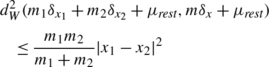
  We merge the particles that add the smallest error first and then continue merging until d _W (μ _N ,μ _merged )<0.15d _W (μ _N ,μ). This has the overall effect of shifting the histogram (taken over all images) of the approximation error to the right, where the inequality is used in the sense of the available upper bound on the distance (Observation 3 and the estimate above) and not the actual distance. This ensures that the final error for each image after merging is around 1.15d _W (μ _N ,μ).

• 8. Finally, while the two steps above seek to find a good particle approximation for each image, with N particles or more, the final step is designed to make the particle approximation error more uniform for all images in a given dataset. For a set of images I ₁,I ₂,…,I _M , we estimate the average transportation error, E _avg , between each digital image and its approximation, as well as standard deviation τ of the errors. We set E _small =E _avg −0.5∗τ and E _big =E _avg +0.5∗τ.

  • For images that have bigger error than E _big , we split the particles as in Step 6 until the error for those images are less than E _big .

  • For images that have smaller error than E _small , we merge nearby particles instead as in Step 7. The procedure we apply is to merge the particles that add the smallest error first and then continue merging until d _W (μ,μ _merged )≥E _small .

References

Ambrosio, L., Gigli, N., & Savaré, G. (2008). Lectures in mathematics ETH zürich. Gradient flows in metric spaces and in the space of probability measures (2nd ed.). Basel: Birkhäuser.
Angenent, S., Haker, S., & Tannenbaum, A. (2003). Minimizing flows for the Monge-Kantorovich problem. SIAM Journal on Mathematical Analysis, 35(1), 61–97. (electronic).
Barrett, J. W., & Prigozhin, L. (2009). Partial L 1 Monge-Kantorovich problem: variational formulation and numerical approximation. Interfaces and Free Boundaries, 11(2), 201–238.
Beg, M., Miller, M., Trouvé, A., & Younes, L. (2005). Computing large deformation metric mappings via geodesic flows of diffeomorphisms. International Journal of Computer Vision, 61(2), 139–157.
Benamou, J. D., & Brenier, Y. (2000). A computational fluid mechanics solution to the Monge-Kantorovich mass transfer problem. Numerische Mathematik, 84(3), 375–393.
Bengtsson, E. (1999). Fifty years of attempts to automate screening for cervical cancer. Medical Imaging Technology, 17, 203–210.
Bishop, C. M. (2006). Pattern recognition and machine learning (information science and statistics). Berlin: Springer.
Blum, H., et al. (1967). A transformation for extracting new descriptors of shape. In Models for the perception of speech and visual form (Vol. 19, pp. 362–380).
Boland, M. V., & Murphy, R. F. (2001). A neural network classifier capable of recognizing the patterns of all major subcellular structures in fluorescence microscope images of hela cells. Bioinformatics, 17(12), 1213–1223.
do Carmo, M. P. (1992). Riemannian geometry. Mathematics: theory & applications. Boston: Birkhäuser Boston. Translated from the second Portuguese edition by Francis Flaherty.
Chefd’hotel, C., & Bousquet, G. (2007). Intensity-based image registration using earth mover’s distance. Proceedings of SPIE, vol. 6512, p. 65122B.
Delzanno, G. L., & Finn, J. M. (2010). Generalized Monge-Kantorovich optimization for grid generation and adaptation in L p . SIAM Journal on Scientific Computing, 32(6), 3524–3547.
Dialynas, G. K., Vitalini, M. W., & Wallrath, L. L. (2008). Linking heterochromatin protein 1 (hp1) to cancer progression. Mutation Research, 647(1–2), 13–20.
Fisher, R. A. (1936). The use of multiple measurements in taxonomic problems. Annals of Eugenics, 7, 179–188.
Gardner, M., Sprague, B., Pearson, C., Cosgrove, B., Bicek, A., Bloom, K., Salmon, E., & Odde, D. (2010). Model convolution: a computational approach to digital image interpretation. Cellular and Molecular Bioengineering , 3(2), 163–170.
Grauman, K., & Darrell, T. (2004). Fast contour matching using approximate earth mover’s distance. In Proceedings of the 2004 IEEE computer society conference on computer vision and pattern recognition, CVPR 2004.
Haber, E., Rehman, T., & Tannenbaum, A. (2010). An efficient numerical method for the solution of the L 2 optimal mass transfer problem. SIAM Journal on Scientific Computing, 32(1), 197–211.
Haker, S., Zhu, L., Tennenbaum, A., & Angenent, S. (2004). Optimal mass transport for registration and warping. International Journal of Computer Vision, 60(3), 225–240.
Kong, J., Sertel, O., Shimada, H., BOyer, K. L., Saltz, J. H., & Gurcan, M. N. (2009). Computer-aided evaluation of neuroblastoma on whole slide histology images: classifying grade of neuroblastic differentiation. Pattern Recognition, 42, 1080–1092.
Ling, H., & Okada, K. (2007). An efficient earth mover’s distance algorithm for robust histogram comparison. In IEEE transactions on pattern analysis and machine intelligence (pp. 840–853).
Lloyd, S. P. (1982). Least squares quantization in pcm. IEEE Transactions on Information Theory, 28(2), 129–137.
Loo, L., Wu, L., & Altschuler, S. (2007). Image-based multivariate profiling of drug responses from single cells. Nature Methods, 4(5), 445–454.
Methora, S. (1992). On the implementation of a primal-dual interior point method. SIAM Journal on Scientific and Statistical Computing, 2, 575–601.
Miller, M. I., Priebe, C. E., Qiu, A., Fischl, B., Kolasny, A., Brown, T., Park, Y., Ratnanather, J. T., Busa, E., Jovicich, J., Yu, P., Dickerson, B. C., & Buckner, R. L. (2009). Collaborative computational anatomy: an mri morphometry study of the human brain via diffeomorphic metric mapping. Human Brain Mapping, 30(7), 2132–2141.
Moss, T. J., & Wallrath, L. L. (2007). Connections between epigenetic gene silencing and human disease. Mutation Research, 618(1–2), 163–174.
Orlin, J. B. (1993). A faster strongly polynomial minimum cost flow algorithm. Operations Research, 41(2), 338–350.
Pele, O., & Werman, M. (2008). A linear time histogram metric for improved sift matching. In ECCV.
Pele, O., & Werman, M. (2009). Fast and robust earth mover’s distances. In Computer vision, 2009 IEEE 12th international conference on (pp. 460–467). New York: IEEE Press.
Pincus, Z., & Theriot, J. A. (2007). Comparison of quantitative methods for cell-shape analysis. Journal of Microscopy , 227(2), 140–156.
Rohde, G. K., Ribeiro, A. J. S., Dahl, K. N., & Murphy, R. F. (2008). Deformation-based nuclear morphometry: capturing nuclear shape variation in hela cells. Cytometry, 73(4), 341–350.
Roweis, S. T., & Saul, L. K. (2000). Nonlinear dimensionality reduction by locally linear embedding. Science, 290(5500), 2323–2326. doi:10.1126/science.290.5500.2323.
Rubner, Y., Tomassi, C., & Guibas, L. J. (2000). The earth mover’s distance as a metric for image retrieval. International Journal of Computer Vision, 40(2), 99–121.
Rueckert, D., Frangi, A. F., & Schnabel, J. A. (2003). Automatic construction of 3-d statistical deformation models of the brain using nonrigid registration. IEEE Transactions on Medical Imaging, 22(8), 1014–1025.
Shamir, L. (2009). Automatic morphological classification of galaxy images. Monthly Notices of the Royal Astronomical Society.
Shirdhonkar, S., & Jacobs, D. (2008). Approximate earth mover’s distance in linear time. In Proceedings of the 2008 IEEE computer society conference on computer vision and pattern recognition, CVPR 2008.
Stegmann, M., Ersboll, B., & Larsen, R. (2003). Fame—a flexible appearance modeling environment. IEEE Transactions on Medical Imaging, 22(10), 1319–1331.
Tenenbaum, J. B., de Silva, V., & Langford, J. C. (2000). A global geometric framework for nonlinear dimensionality reduction. Science, 290(5500), 2319–2323. doi:10.1126/science.290.5500.2319.
Vaillant, M., Miller, M., Younes, L., & Trouvé, A. (2004). Statistics on diffeomorphisms via tangent space representations. NeuroImage, 23, S161–S169.
Villani, C. (2003). Graduate studies in mathematics: Vol. 58. Topics in optimal transportation. Providence: Am. Math. Soc..
Villani, C. (2009). In Grundlehren der Mathematischen Wissenschaften [Fundamental principles of mathematical sciences]: Vol. 338. Optimal transport. Berlin: Springer. doi:10.1007/978-3-540-71050-9.
Wang, W., Mo, Y., Ozolek, J. A., & Rohde, G. K. (2011). Penalized fisher discriminant analysis and its application to image-based morphometry. Pattern Recognition Letters, 32(15), 2128–2135.
Wang, W., Ozolek, J., & Rohde, G. (2010). Detection and classification of thyroid follicular lesions based on nuclear structure from histopathology images. Cytometry Part A, 77(5), 485–494.
Wang, W., Ozolek, J., Slepčev, D., Lee, A., Chen, C., & Rohde, G. (2011). An optimal transportation approach for nuclear structure-based pathology. IEEE Transactions on Medical Imaging, 30(3), 621–631.
Yang, L., Chen, W., Meer, P., Salaru, G., Goodell, L., Berstis, V., & Foran, D. (2009). Virtual microscopy and grid-enabled decision support for large scale analysis of imaged pathology specimens. IEEE Transactions on Information Technology in Biomedicine, 13(4), 636–644.
Acknowledgements
The authors wish to thank the anonymous reviewers for helping significantly improve this paper. W. Wang, S. Basu, and G.K. Rohde acknowledge support from NIH grants GM088816 and GM090033 (PI GKR) for supporting portions of this work. D. Slepčev was also supported by NIH grant GM088816, as well as NSF grant DMS-0908415. He is also grateful to the Center for Nonlinear Analysis (NSF grant DMS-0635983 and NSF PIRE grant OISE-0967140) for its support.
Author information
Authors and Affiliations
Corresponding author