Shadow Areas Robust Matching Among Image Sequence in Planetary Landing

Abstract

In this paper, an approach for robust matching shadow areas in autonomous visual navigation and planetary landing is proposed. The approach begins with detecting shadow areas, which are extracted by Maximally Stable Extremal Regions (MSER). Then, an affine normalization algorithm is applied to normalize the areas. Thirdly, a descriptor called Multiple Angles-SIFT (MA-SIFT) that coming from SIFT is proposed, the descriptor can extract more features of an area. Finally, for eliminating the influence of outliers, a method of improved RANSAC based on Skinner Operation Condition is proposed to extract inliers. At last, series of experiments are conducted to test the performance of the approach this paper proposed, the results show that the approach can maintain the matching accuracy at a high level even the differences among the images are obvious with no attitude measurements supplied.

1 Introduction

Communication delay between lander and earth in planetary exploration has been considered to be an issue in future’s planetary mission (Yu et al. 2014), the mission should require autonomous navigation for motion estimation and hazard avoidance to get close to the landing site of planet (Epp et al. 2007; Johnson et al. 2008). However, current traditional EDL (Entry, Descent, and Landing) are far from the capability (Yu et al. 2014; Pham et al. 2010a, b).

Autonomous optical navigation can provide positions of the lander by matching landmarks that were obtained from descent images (Yu et al. 2014; Johnson and Montgomery 2008). Position estimation of lander can be divided into two parts (Johnson and Montgomery 2008): Global position estimation and Velocity estimation. Global position estimation matches the landmarks which were obtained in the process of descent with the database in which the landmarks’ absolute positions are stored. The database was constructed during orbital reconnaissance. Landmarks are usually chosen from the terrains that can be easy detected, and the terrains are widely spread on the surface of planet, such as craters, whose shape often follows the well-known geometric model of ellipse, and they can be detected under a wide range of illumination conditions without scene scale and relative orientation between camera and the surface (Wetzler et al. 2005; Cheng et al. 2003; Cheng and Ansar 2005). However, some craters without regular shape may be hard to be detected, and the areas that around the landing sites are not sure that there have enough craters to enable landmarks matching. Different from Global position estimation, velocity estimation is based on matching landmarks among image sequence, and the approach can be split into two categories based on the types of required input: Descent Image Motion Estimation Subsystem (DIMES; Johnson et al. 2007; Trawny et al. 2007) and Structure from Motion (SFM; Bouguet and Perona 1995; Montgomery et al. 2006; Ansar and Cheng 2010). DIMES takes the descent images, attitude and altitude estimates as the input, the output is horizontal velocity, which can be calculated by correlating images patches from one descent image to the next, during the process, each descent image is needed to rectified to the local frame according to the change of attitude and altitude, the approach has been tested successfully in Mars Exploration Rover landings (Johnson et al. 2008). However, the output is just horizontal velocity, angular rate cannot be estimated. SFM takes the descent images and altitudes estimates as the input, during the phase of descent, multiple image features are detected and matched from one descent image to the next one, the output is not just horizontal velocity, angular rate can also been estimated, and the approach based on SFM has been tested in a helicopter during autonomous landing (Montgomery et al. 2006). However, this is still a challenge to achieve robust matching among descent images with large difference of viewpoint under no attitude measurement supplied at present. Shi-Tomasi-Kanad (Benedetti and Perona 1998; Shi and Tomasi 1994; Johnson et al. 1999) and Harris and Stephens (1988) are often likely to be adopted as the corner detection, however, as mentioned in (Montgomery et al. 2006), it is possible to track their features when the change of attitude is less than 10° in the roll, 20° in pitch, and 20% in altitude, in addition, the approach is sensitivity to noise. Sift (Lowe 2004) and Surf (Bay et al. 2008) may have better robust performance, however, it is not good enough when the difference of viewpoint is larger than 30°.

Shadow areas, which are formed by different kinds of terrain can be easily detected and are widely distributed on the surface of planets, they are usually used for hazards detection and avoidance (HDA; Johnson et al. 2008). Unlike Harris and Sift, shadow areas’ shapes are stable in illumination, and their outlines can be considered as a kind of features to add more information about the areas. However, few research works published take shadow areas as the landmarks to track among descent images during lander approaching to the landsite at current time. Therefore, an approach that is based on robust matching shadow areas is proposed in this paper, not only can the approach deal with the issue of SFM as mentioned above, but also can maintain the matching accuracy at a high level even the difference of viewpoint is large without the information of attitude’s change that is obtained by attitude measuring equipment.

For describing the approach, the rest of this paper is organized as follows. Section 2 introduces a method that combine Binary Threshold for Shadow Areas (this paper proposed) with MSER to extract shadow areas that with stable shape. Section 3 is the main part, we introduce an affine normalization to normalize every shadow area, and then a proposed descriptor MASIFT is introduced for features extraction. In Sect. 4, SKINNER-RANSAC is proposed to eliminate mismatched pairs, and then mismatched pairs rectified by estimation correct homography (Agarwal et al. 2005). Performance of the approach this paper proposed is discussed by comparing with the existing method in Sect. 5. Finally, conclusion are given in Sect. 6. The sketch of the approach is shown in Fig. 1.

Fig. 1

Sketch of the proposed approach

2 Shadow Areas

As we know, camera, which the lander installed takes photos of planetary surface during descent, so, the shadow areas extracted should be always be tracked if they are taken as the landmarks. However, the grey values of shadow areas are very likely varies with illumination conditions’ change, and the illumination conditions’ change attributes to the change of lander’s position in the process of landing, furthermore, when the lander is at a long distance to the surface of planet, shadow areas and dark space will co-exist together in a image as shown in (a) of Fig. 2, which will be discussed in bellow, the grey value of dark space is darker than shadow areas, that will make shadow areas extraction much more difficult in this situation. Therefore, extracting shadow areas with effective method is crucial in our proposed approach. In this section, we introduce a new method aim at extracting shadow areas from planetary surface image, the method can be divided into three parts. Firstly, the notion “Isolated Intensity” will be introduced, and the application of isolated intensity will improve the accuracy of shadow areas detection. Secondly, Binary Threshold for Shadow Areas (BTSA) will be introduced to determine the global threshold of shadow areas. Thirdly, Maximally Stable Extremal Regions (MSER) will be applied to get the shadow areas with stable shapes.

Fig. 2

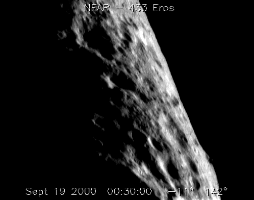
Two images taken from 433Eros. a Long distance (NASA PHOTO near_20000919_large_anim); b close distance (NASA PHOTO near_20000511)

2.1 Isolated Intensity

There are two images of 433 Eros, which were taken at different positions as shown in Fig. 2. The image in (a) is taken at a long distance from the asteroid, carefully observe the image, It can be seen that nearly 2/5 that of the image is occupied by the dark space that its intensity lies within the range from 0 to 10, however, the intensity of shadow areas lies within the range from 0 to 60, therefore, the part of the space may influence the detection of shadow areas in view of using global threshold. In real application, the part of dark space in image can be seen as the background and it can be extracted by analyzing the imager (CCD noise) and background noise, however, some areas with lower intensities cannot be seen as background as shown in (b) of Fig. 2, observe it carefully, we can found that there have three huge craters, and the grey of the three huge craters lies within the range from 0 to 5, however, the intensities of small shadow areas that surrounded the three huge craters lies within the range from 6 to 36, so, it will be hard to extract shadow areas by current algorithm of global threshold, such as OSTU (Ohtsu 1979).

Therefore, a type of intensity that with large number of pixels is concentrated here to deal with the issue above, and we call this type of intensity “Isolated Intensity”. In our work, we use least square method to detect them, now we take images of Fig. 2 as the examples to explain this method. We found 10-degree equation in one variable can be applied to fit most of histogram after a large number of experiments. Figure 3 displays the histograms and their fitting curves by least square, it can be found that both of the histogram are fitted well, however, the different between histogram and fitted curve is obvious when the intensity within the range from 0 to 7 in (a), and the intensity within the range from 0 to 10 in (b). The distance from histogram to the fitted curve is displayed in Fig. 4, in which, most parts are concentrated in the areas that surround 0 except the intensity within the range from 0 to 7 in (a), and the intensity within the range from 0 to 10 in (b). Figure 5 displays the distribution of number of pixels in different distances, the distances approximately obey the normal distribution. So, the isolated intensity can be detected according to the normal distribution of number of pixels in different distances, a method of isolated intensity detection is introduced in Lemma 1 as shown in below.

Fig. 3

The histogram and its fitted curve for the images in Fig. 2. a The left one in Fig. 2; b the right one in Fig. 2

Fig. 4

Distance from histograms to the fitted curve. a The left one in Fig. 3; b the right one in Fig. 3

Fig. 5

The total number of pixels in different distance. a The left one in Fig. 4; b The right one in Fig. 4

Let $S$ denote a set that contains the number of each intensity’s pixel, $s(i) \in S(i = 0,1,\, \ldots ,\,255),$ which denotes the number of pixels about intensity $i$. Suppose $\ell$ is the fitting cure, and $\ell (i) (i = 0,1,\, \ldots ,\,255)$ is the value of $\ell$ that corresponds to $s(i) (i = 0,1,\, \ldots ,\,255)$.

Lemma 1

Let $d(i) = s(i) - \ell (i)(i = 0,1, \ldots ,255)$ , if $j$ is the isolated intensity, there will be:

$$d(j) > 0,\,\frac{1}{{\sqrt { 2\uppi} \sigma }}{\text{e}}^{{\frac{{{ - (}d (j ) { - }\mu )^{2} }}{{2\sigma^{2} }}}} \ll \overline{p}$$

(1)

where

$$\mu = \frac{1}{256}\sum\limits_{i = 0}^{25 5} {d (i )}$$

(2)

$$\sigma = \sqrt {\frac{1}{256}\sum\limits_{i = 0}^{25 5} { (d (i )} { - }\mu )^{2} }$$

(3)

$$\overline{p} = \frac{1}{256}\sum\limits_{i = 0}^{25 5} {\frac{1}{{\sqrt { 2\uppi} \sigma }}{\text{e}}^{{\frac{{{ - (}d (i ) { - }\mu )^{2} }}{{2\sigma^{2} }}}} }$$

(4)

Proof

Suppose $d(j)$ is the distance from $s(j)$ to $\ell (j)$. If $d (j )< 0$, the number of pixels with intensity $j$ cannot affect the detection of shadow areas, however, if $d (j )> 0$, $j$ may be the isolate intensity, the distances $d(i)(i = 0,1 \cdots 255)$ approximately obey the normal distribution $N (\mu ,\sigma )$, let $\overline{p}$ denote the average probability of $d$, if $j$ is the isolated intensity in $S$, the probability of $d(j)$ must be smaller than $\overline{p}$.

In this paper, if $\frac{1}{{\sqrt { 2\uppi} \sigma }}{\text{e}}^{{\frac{{{ - (}d (j ) { - }\mu )^{2} }}{{2\sigma^{2} }}}} \le {{\overline{p} } \mathord{\left/ {\vphantom {{\overline{p} } { 1 0}}} \right. \kern-0pt} { 1 0}}$ and $d (j )> 0$, $j$ can be considered as the isolated intensity.

After the detection of isolated intensities, they are replaced by the average grey of the image as shown in Fig. 6.

Fig. 6

Isolated intensities replaced by the average grey of respective image

2.2 Threshold

Binary Threshold for Shadow Areas (BTSA) is proposed for the calculation of threshold of shadow areas here. The method can be organized into 8 steps:

Step 1 Calculate the average intensity.

$$\overline{f} = \frac{1}{M \times N}\sum\limits_{x = 1}^{M} {\sum\limits_{y = 1}^{N} {f(x,y)} }$$

(5)

where $M$ and $N$ are image’s height and width respectively, $f(x,y)$ is the intensity at $(x ,y )$.

Step 2 Obtain the vector $b$ in descent, the vector contains the pixels that with their intensities are less than $\overline{f}$.

$$b:b(i) \le \overline{f} \;{\text{and}}\;b(i + 1) \ge b(i)$$

(6)

where $i = 1,2, \ldots ,n_{1}$, $n_{1}$ is the number of pixels, and intensities of the pixels are less than $\overline{f}$.

Step 3 Let $b$ subtract $\overline{f}$ and get a new vector $b^{\prime}$.

$$b^{\prime} (i) = b(i) - \overline{f}$$

(7)

Step 4 Calculate the change rate, and its average value $\overline{{v_{1} }}$ and $\overline{{v_{2} }}$.

$$v:v(i) = b^{\prime} ((i + 1) \times T) - b^{\prime} (i \times T),\;T = M \times N/\text{Im} {\text{g}}_{\text{intensity}}$$

(8)

$$\overline{v} = \frac{1}{{n_{1} - 1}}\sum\limits_{i = 1}^{{n_{1} - 1}} {v(i)}$$

(9)

where $i = 1,2 \cdots ,n_{1} /T$, $T$ is the step length, $\text{Im} {\text{g}}_{{\text{int} {\text{ensity}}}} = 256$.

Step 5 Obtain the maximum position $L$.

$$L = \hbox{max} (i|v(i) > \overline{v} )$$

(10)

where $i = 1,2, \ldots ,n_{1} /T$.

Step 6 Calculate the length scale $p$.

$$p = L/(n_{1} - 1)$$

(11)

Step 7 Calculate the standard deviation $f$:

$$f = \sqrt {\sum\limits_{i = 1}^{{n_{1} \times p}} {\varvec{b} (i )^{2} } / (n_{1} \times p)}$$

(12)

Step 8 Obtain the threshold $\alpha$ of global shadow areas:

$$\alpha = \overline{f} - f$$

(13)

The comparison of shadow areas detected between the method this section proposed and OSTU is shown in Fig. 7. Observe (a), we find that most shadow areas can be extracted after the isolated intensities detected, while, few shadow areas can be detected by OSTU only. Observe (b), although the different between the two methods is not obviously, it is still can be found that shadow areas with smaller size can be detected after isolated intensities detected. As we know that no matter what size it is, any shadow area can be considered as a hazard or landmark (Yu et al. 2014), so, the detection of isolated intensity is significance for detection shadow areas on the planetary surface.

Fig. 7

Comparison between proposed method and OSTU in Fig. 2

2.3 Maximally Stable Extremal Regions

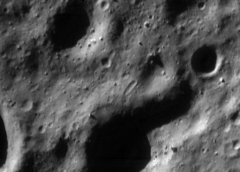
As we have mentioned above, extracting shadow areas with effective method is crucial in our proposed approach. Thanks to Maximally Stable Extremal Regions (MSER; Matas et al. 2004), which has been considered as the best area extraction method at present. This method of extracting a comprehensive number of corresponding image elements contributes to the wide-baseline matching, and it has led to better stereo matching and object recognition algorithms. So, we use MSER as the tools to detect the stable regions in shadow areas. We chose several images with different types of terrain to as the targets to investigate MSER’s performance as shown in Fig. 8a–e are taken from 433 Eros at different heights, and (f) is taken from Moon at the location: 8°57′8.88″S, 15°27′19.26″E. The threshold of shadow areas are obtained by the method that explained in Sects. 2.1, 2.2. Shadow areas with stable shapes extracted as shown in Fig. 9, the results reveals that most shadow areas on the planetary surface can be detected by the method combine isolated intensities detection with MSER.

Fig. 8

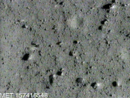
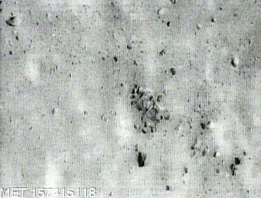
Several images taken from 433 Eros and Moon. a–e Images that are taken from 433 Eros (NASA PHOTO: near_flyover_anim_large, near_20000919_large_anim, The final approach, near_descent_157416548, near_descent_157415118); f an image that are taken from Moon at the location: 8°57′8.88″S, 15°27′19.26″E

Fig. 9

Stable shadow areas marked with ellipses. a–b Fig. 2; c–h Fig. 8

3 Robust Matching

Consider the attitude of spacecraft is constantly changing in the process of landing, the images must be varies with the change of viewpoint, rotation and scale. How to guarantee the performance of robust matching shadow areas among descent images that their differences of viewpoint are large is the key point in the approach this paper proposed. Therefore we introduce a method to tackle this issue as mentioned above, the method can be divided into 3 steps as shown in bellow, and the details of these steps will be explained in this section.

• Step 1 Extract each shadow area detected from image into small pieces of cube.

• Step 2 Normalize the shadow areas extracted into the same size, direction and shape according to their geometric characteristics.

• Step 3 A new descriptor called “Multiple Angles SIFT” is proposed for catching more features of shadow area.

3.1 Shadow Areas Segmentation

We hope all the shadow areas detected should be cut out, however, account for the extracting the features of shadow areas, which will be discussed in the next section, the one located at the edge of image cannot be cut out due to that they cannot be extract features completely, that will influence the matching performance. Therefore, the produce of shadow areas segmentation should be specified. Let $S_{adow}$ denote a shadow area as shown in Fig. 10, $H_{\hbox{min} }$ and $H_{\hbox{max} }$ are the minimum and maximum values on the horizontal ordinate of the image, respectively, at the same time, $V_{\hbox{min} }$ and $V_{\hbox{max} }$ are the minimum and maximum value on the vertical ordinate of the image respectively, and the size of image is $M \times N$, the shadow areas cut out should be satisfied with the conditional formula as shown in Eq. (14).

Fig. 10

Example of shadow area extraction

$$\left\{ {\begin{array}{*{20}c} {H_{\hbox{max} } + H_{mid} \le M} \\ {H_{\hbox{min} } - H_{mid} \ge 0} \\ {V_{\hbox{max} } + V_{mid} \le N} \\ {V_{\hbox{min} } - V_{mid} \ge 0} \\ \end{array} } \right.$$

(14)

3.2 Normalization

In this section, three parts are introduced: shape normalization, size normalization and rotation normalization.

3.2.1 Shape Normalization

Shape normalization is introduced in (Lu et al. 2010; Pei and Lin 1995), and the main steps can be depicted as follows:

Step 1 Compute the covariance matrix $M$ of the given shadow area which locates in the shadow sub graph.

Step 2 Construct a rotational matrix $E$ with the eigenvectors of $M$ to align the coordinates.

Step 3 Construct a scaling matrix $W$ to rescale the coordinates by the eigenvalues of $M$.

Step 4 Suppose $[x,y]$ is a location of a point in the original image, $[\overline{x} ,\overline{y} ]$ is the correspond location in the transformed image, $[C_{x} ,C_{y} ]$ is the center of the minimum bounding rectangle as shown in Fig. 10. The normalized shadow subgraph can be obtained by:

$$\left[ {\begin{array}{*{20}c} {\overline{x} } \\ {\overline{y} } \\ \end{array} } \right] = W \times E \times \left[ {\begin{array}{*{20}c} {x - C_{x} } \\ {y - C_{y} } \\ \end{array} } \right]$$

(15)

After shape normalization, a square area that called ‘square normalized shadow area’ contains the shadow area should be extracted with the size of the area larger than the shadow area’s minimum bounding rectangle. Let $S_{adow}^{n}$ denote the normalized shadow area in the normalized shadow sub graph, $H_{\hbox{min} }^{n}$ denote the minimum value on the horizontal ordinate, $H_{\hbox{max} }^{n}$ denote the maximum value on the horizontal ordinate, $V_{\hbox{min} }^{n}$ denote the minimum value on the vertical coordinate, and $V_{\hbox{max} }^{n}$ denote the maximum value on the vertical coordinate, the side length in minimum bounding rectangle can be obtained as shown in Fig. 11, in which, $H_{length}^{n} = H_{\hbox{max} }^{n} - H_{\hbox{min} }^{n}$, $V_{length}^{n} = V_{\hbox{max} }^{n} - V_{\hbox{min} }^{n}$. In fact, $H_{length}^{n} \approx V_{length}^{n}$. Let $Dia^{n} = \sqrt[2]{{(H_{length}^{n} )^{2} + (V_{length}^{n} )^{2} }}$, which is side length of the square normalized shadow area, and the center of the minimum bounding rectangle of the shadow area is determined to be the center of the square normalized shadow area.

Fig. 11

The square area that contained the shadow area

3.2.2 Size Normalization

The side length in different square normalized shadow areas should be made to be the same, which can be depicted as a term of an equation:

$$L = \frac{{L_{1} + L_{2} }}{2}$$

(16)

where $L$ is the unified side length, $L_{1} = \frac{1}{{n_{1} }}\sum\nolimits_{i = 1}^{{n_{1} }} {l_{i}^{1} }$ and $L_{2} = \frac{1}{{n_{2} }}\sum\nolimits_{j = 1}^{{n_{2} }} {l_{j}^{2} }$, $n_{1}$ is the number of the normalized shadow areas in the first image, and $n_{2}$ is the number of the normalized shadow areas in the second image.

3.2.3 The Rotation Normalization

Principal orientation that introduced in (Schmid and Mohr 1997) should be conformed for each normalized shadow areas, and rotate the areas to the principal orientation. In this section, we make use of orientation histogram to determine the principal orientation, firstly, for each normalized shadow area, get the orientation histogram with 36 bins which covers 360 degrees, secondly, find the highest peak of the histogram, any other local peaks that larger than 80% of the highest peaks can also be assigned to the principal orientation.

Let $SL$ denote the normalized shadow area that have the unified size.$SL$ must be smoothed by Gaussian function $G(x,y,\delta )$ before the formation of orientation histogram,$\delta$ is a scaling function, and a formula is designed for $\delta$:

$$\delta = \hbox{min} (b^{{\log_{2} (L_{pre} /L + 1)}} ,b)$$

(17)

where $b$ is the maximum value of $\delta$, $L_{pre}$ is the side length of the shape normalized shadow area before size normalized, and $L$ is the side length of normalized shadow area after size normalized. Suppose $b = 4$, the value of $L_{pre} /L$ is between 0.01 and 10, if the step length is 0.01, $\delta$ varies with the change of $L_{pre} /L$, which is illustrated in Fig. 8, we can found that $\delta$ is between 1 and 4, $\delta$ can be maintained at the maximum value when $L_{pre} /L$ is larger than 1. The relation is shown in Fig. 12.

Fig. 12

The relation between $\delta$ and $L_{pre} /L$

3.3 MA-SIFT (Multiple Angles Sift)

Many descriptors have been proposed for describing key points or areas, such as SIFT, SURF, PCA-SIFT (Ke and Sukthankar 2004) and GLOH (Moreno et al. 2009), etc. However, usually the sub regions of the existing descriptors are fixed with no any changed at all in the process of features extraction, which may cause the features extraction imperfectly. In the next part, we will prove the judgment by theoretical derivation and group of experiment.

Lemma 2

The influence of the regions with obvious difference can be reduced by the rotation of coordinate system in anticlockwise with the angle smaller than $\pi /4$.

Proof

Suppose there is a descriptor, which is made up of four sub regions, they are $A$, $B$, $C$ and $D$, as shown in (a) of Fig. 13. Now, assume the descriptor locate at the same area of a couple of matched images, and the sub regions are similar expect the sub region $C$, so, the features extracted by the descriptor can be expressed in Eqs. (18, 19):

$$A_{l} :a_{1} ,a_{2} ,\, \ldots ,\,a_{m} ;\;B_{l} :b_{1} ,b_{2} ,\, \ldots ,\,b_{m} ;\;C_{l} :c_{1} ,c_{2} ,\, \ldots ,\,c_{m} ;\;D_{l} :d_{1} ,d_{2} ,\, \ldots ,\,d_{m}$$

(18)

$$\left\{ {\begin{array}{*{20}c} {A_{r} :a_{1} + fn(a_{1} )/t,a_{2} + fn(a_{2} )/t,\, \cdots ,\,a_{m} + fn(a_{m} )/t} \\ {B_{r} :b_{1} + fn(b_{1} )/t,b_{2} + fn(b_{2} )/t,\, \cdots ,\,b_{m} + fn(b_{m} )/t} \\ {C_{r} :c_{1} + fn(c_{1} )/k,c_{2} + fn(c_{2} )/k,\, \cdots ,\,c_{m} + fn(c_{m} )/k} \\ {D_{r} :d_{1} + fn(d_{1} )/t,d_{2} + fn(d_{2} )/t,\, \cdots ,\,d_{m} + fn(d_{m} )/t} \\ \end{array} } \right.$$

(19)

where $A_{l}$, $B_{l}$, $C_{l}$ and $D_{l}$ are the sub regions of descriptor in the first image, at the same time, $A_{r}$, $B_{r}$, $C_{r}$ and $D_{r}$ are the sub regions of descriptor in the corresponded image. Suppose each sub region can extracted m features, then, $a_{i} (i = 1,2,\, \ldots ,\,m)$ are the features in sub region $A_{l}$, $b_{i} (i = 1,2,\, \ldots ,\,m)$ are the features in sub region $B_{l}$, $c_{i} (i = 1,2,\, \ldots ,\,m)$ are the features in sub region $C_{l}$, and $d_{i} (i = 1,2,\, \ldots ,\,m)$ are the features in sub region $D_{l}$. For simulating the difference of the same features between the matched sub regions, we design a float function for each feature in the sub regions of the matched images. For example, as shown in Eq. (19), $f \times n(a_{1} )/t$ is the float function of $a_{1}$,$f$ is a constant, which can be the average of features in the 4 sub regions, and $n(a_{1} )$ is a Gaussian distribution with 0 as the mean, and 0.5 as its standard deviation, and $t$ means the factor of reduced in scale, this factor often larger than 10, which ensure the similar of the same sub region in matched images. However, the factor $k$ should be smaller than $t$, and it should be satisfied the inequality: $10 \times k \le t$, which ensure the features of the sub region are more different compare with other three parts. Based on the assumption as mentioned above, distance of descriptor with the coordinate system have no rotation in the two matched images is shown in Eq. (20):

$$\begin{aligned} d & = \sqrt {\sum\limits_{i = 1}^{m} {(a_{i} - a_{i} + fn(a_{i} )/t)^{2} } + \sum\limits_{i = 1}^{m} {n^{2} (d_{i} )} \sum\limits_{i = 1}^{m} {(b_{i} - b_{i} + fn(b_{i} )/t)^{2} } + \sum\limits_{i = 1}^{m} {(c_{i} - c_{i} + fn(c_{i} )/k)^{2} } + \sum\limits_{i = 1}^{m} {(d_{i} - d_{i} + fn(d_{i} )/t)^{2} } } \\ & = \sqrt {f^{2} /t^{2} (\sum\limits_{i = 1}^{m} {n^{2} (a_{i} )} + + \sum\limits_{i = 1}^{m} {n^{2} (b_{i} )} + \sum\limits_{i = 1}^{m} {n^{2} (d_{i} ))} + f^{2} /k^{2} \sum\limits_{i = 1}^{m} {n^{2} (c_{i} )} } \\ \end{aligned}$$

(20)

Fig. 13

Descriptor and its form of coordinate system rotation. a The sub regions with the coordinate system have no rotation; b the sub regions after coordinate system rotate in anticlockwise with an angle of $\alpha$

Now, suppose the coordinate system rotates in clockwise with an angle of $\alpha$, as shown in (b) of Fig. 13, then, we can get a group of new parts: $A^{\prime}$, $B^{\prime}$, $C^{\prime}$, $D^{\prime}$. So, the features of the sub regions can be expressed as shown in Eqs. (21, 22):

$$\left\{ {\begin{array}{*{20}c} {A_{l}^{\prime} :\left(\frac{\pi - 4\alpha }{\pi }\right)a_{1} + \frac{4\alpha }{\pi }b_{1} ,\left(\frac{\pi - 4\alpha }{\pi }\right)a_{2} + \frac{4\alpha }{\pi }b_{2} , \cdots \left(\frac{\pi - 4\alpha }{\pi }\right)a_{m} + \frac{4\alpha }{\pi }b_{m} } \\ {B_{l}^{\prime} :\left(\frac{\pi - 4\alpha }{\pi }\right)b_{1} + \frac{4\alpha }{\pi }c_{1} ,\left(\frac{\pi - 4\alpha }{\pi }\right)b_{2} + \frac{4\alpha }{\pi }c_{2} , \cdots \left(\frac{\pi - 4\alpha }{\pi }\right)b_{m} + \frac{4\alpha }{\pi }c_{m} } \\ {C_{l}^{\prime} :\left(\frac{\pi - 4\alpha }{\pi }\right)c_{1} + \frac{4\alpha }{\pi }d_{1} ,\left(\frac{\pi - 4\alpha }{\pi }\right)c_{2} + \frac{4\alpha }{\pi }d_{2} , \cdots \left(\frac{\pi - 4\alpha }{\pi }\right)c_{m} + \frac{4\alpha }{\pi }d_{m} } \\ {D_{l}^{\prime} :\left(\frac{\pi - 4\alpha }{\pi }\right)d_{1} + \frac{4\alpha }{\pi }a_{1} ,\left(\frac{\pi - 4\alpha }{\pi }\right)d_{2} + \frac{4\alpha }{\pi }a_{2} , \cdots \left(\frac{\pi - 4\alpha }{\pi }\right)d_{m} \frac{4\alpha }{\pi }a_{m} } \\ \end{array} } \right.$$

(21)

$$\left\{ {\begin{array}{*{20}c} \begin{aligned} A_{r}^{\prime} :\frac{\pi - 4\alpha }{\pi }(a_{1} + fn(a_{1} )/t) + \frac{4\alpha }{\pi }(b_{1} + fn(b_{1} )/t),\frac{\pi - 4\alpha }{\pi }(a_{2} + fn(a_{2} )/t) \hfill \\ \quad+ \frac{4\alpha }{\pi }(b_{2} + fn(b_{2} )/t), \cdots \frac{\pi - 4\alpha }{\pi }(a_{m} + fn(a_{m} )/t) + \frac{4\alpha }{\pi }(b_{m} + fn(b_{m} )/t) \hfill \\ \end{aligned} \\ \begin{aligned} B_{r}^{\prime} :\frac{\pi - 4\alpha }{\pi }(b_{1} + fn(b_{1} )/t) + \frac{4\alpha }{\pi }(c_{1} + fn(c_{1} )/k),\frac{\pi - 4\alpha }{\pi }(b_{2} + fn(b_{2} )/t) \hfill \\ \quad+ \frac{4\alpha }{\pi }(c_{2} + fn(c_{2} )/k), \cdots \frac{\pi - 4\alpha }{\pi }(b_{m} + fn(b_{m} )/t) + \frac{4\alpha }{\pi }(c_{m} + fn(c_{m} )/k) \hfill \\ \end{aligned} \\ \begin{aligned} C_{r}^{\prime} :\frac{\pi - 4\alpha }{\pi }(c_{1} + fn(c_{1} )/k) + \frac{4\alpha }{\pi }(d_{1} + fn(d_{1} )/t),\frac{\pi - 4\alpha }{\pi }(c_{2} + fn(c_{2} )/k) \hfill \\ \quad+ \frac{4\alpha }{\pi }(d_{2} + fn(d_{2} )/t), \cdots \frac{\pi - 4\alpha }{\pi }(c_{m} + fn(c_{m} )/k) + \frac{4\alpha }{\pi }(d_{m} + fn(d_{m} )/t) \hfill \\ \end{aligned} \\ \begin{aligned} D_{r}^{\prime} :\frac{\pi - 4\alpha }{\pi }(d_{1} + fn(d_{1} )/t) + \frac{4\alpha }{\pi }(a_{1} + fn(a_{1} )/t),\frac{\pi - 4\alpha }{\pi }(d_{2} + fn(d_{2} )/t) \hfill \\ \quad+ \frac{4\alpha }{\pi }(a_{1} + fn(a_{1} )/t), \cdots \frac{\pi - 4\alpha }{\pi }(d_{m} + fn(d_{m} )/t) + \frac{4\alpha }{\pi }(a_{m} + fn(a_{m} )/t) \hfill \\ \end{aligned} \\ \end{array} } \right.$$

(22)

So, the distance of sub regions can be expressed as shown in Eq. (23):

$$d^{\prime} = \sqrt {R_{1} + R_{2} + R_{3} + R_{4} }$$

(23)

where,

$$R_{1} = \left(\frac{\pi - 4\alpha }{t\pi }\right)^{2} \sum\limits_{i = 1}^{m} {f^{2} n^{2} (a_{i} )} + \left(\frac{4\alpha }{t\pi }\right)^{2} \sum\limits_{i = 1}^{m} {f^{2} n^{2} (b_{i} )} + \frac{8\alpha (\pi - 4\alpha )}{{t^{2} \pi^{2} }}\sum\limits_{i = 1}^{m} {f^{2} n(a_{i} )} n(b_{i} )$$

$$R_{2} = \left(\frac{\pi - 4\alpha }{t\pi }\right)^{2} \sum\limits_{i = 1}^{m} {f^{2} n^{2} (b_{i} )} + \left(\frac{4\alpha }{k\pi }\right)^{2} \sum\limits_{i = 1}^{m} {f^{2} n^{2} (c_{i} )} + \frac{8\alpha (\pi - 4\alpha )}{{tk\pi^{2} }}\sum\limits_{i = 1}^{m} {f^{2} n(b_{i} )} n(c_{i} )$$

$$R_{3} = \left(\frac{\pi - 4\alpha }{k\pi }\right)^{2} \sum\limits_{i = 1}^{m} {f^{2} n^{2} (c_{i} )} + \left(\frac{4\alpha }{t\pi }\right)^{2} \sum\limits_{i = 1}^{m} {f^{2} n^{2} (d_{i} )} + \frac{8\alpha (\pi - 4\alpha )}{{tk\pi^{2} }}\sum\limits_{i = 1}^{m} {f^{2} n(c_{i} )} n(d_{i} )$$

$$R_{4} = \left(\frac{\pi - 4\alpha }{t\pi }\right)^{2} \sum\limits_{i = 1}^{m} {f^{2} n^{2} (d_{i} )} + \left(\frac{4\alpha }{t\pi }\right)^{2} \sum\limits_{i = 1}^{m} {f^{2} n^{2} (a_{i} )} + \frac{8\alpha (\pi - 4\alpha )}{{t^{2} \pi^{2} }}\sum\limits_{i = 1}^{m} {f^{2} n(d_{i} )} n(a_{i} )$$

In general, we can consider that: $n(a_{i} ) \approx n(b_{i} ) \approx n(c_{i} ) \approx n(d_{i} )$, so,

$$\begin{aligned} d^{\prime} & \approx \sqrt {f^{2} /t^{2} (\sum\limits_{i = 1}^{m} {n^{2} (a_{i} )} + \sum\limits_{i = 1}^{m} {n^{2} (d_{i} )} ) + R_{2} + R_{3} } \\ { = }\sqrt {f^{2} /t^{2} (\sum\limits_{i = 1}^{m} {n^{2} (a_{i} )} + \sum\limits_{i = 1}^{m} {n^{2} (b_{i} ) + } \sum\limits_{i = 1}^{m} {n^{2} (d_{i} )} ) + f^{2} /k^{2} \sum\limits_{i = 1}^{m} {n^{2} (c_{i} ) + R_{1}^{\prime} + R_{2}^{\prime} } } \\ \end{aligned}$$

(24)

where

$$R_{1}^{\prime} = \frac{16a(\pi - 4a)}{{tk\pi^{2} }}\sum\limits_{i = 1}^{m} {f^{2} n^{2} (c_{i} )}$$

$$R_{2}^{\prime} = - 8a(\pi - 4a) \left(\frac{1}{{t^{2} \pi^{2} }} + \frac{1}{{k^{2} \pi^{2} }}\right) \sum\limits_{i = 1}^{m} {f^{2} n^{2} (c_{i} )}$$

If $\alpha \le \pi /4$, then

$$\begin{aligned} R_{1}^{\prime} + R_{2}^{\prime} & = - 8a(\pi - 4a)\left(\frac{2tk}{{t^{2} k^{2} \pi^{2} }} + \frac{{k^{2} }}{{t^{2} k^{2} \pi^{2} }} + \frac{{t^{2} }}{{t^{2} k^{2} \pi^{2} }}\right)\sum\limits_{i = 1}^{m} {f^{2} n^{2} (c_{i} )} \\& = - 8a(\pi - 4a)\frac{{(t{ + }k)^{2} }}{{t^{2} k^{2} \pi^{2} }}\sum\limits_{i = 1}^{m} {f^{2} n^{2} (c_{i} )} \le 0 \\ \end{aligned}$$

So, we can get that $d^{\prime} \le d$ under the condition $\alpha \le \pi /4$.

After the theoretical derivation, we will give an example to improve the lemma. The same shadow area that framed with white rectangles in consecutive images is illustrated in Figs. 14, and 15 illustrates their normalized types by the method that described in Sect. 3.2. From Fig. 15, the shadow areas extracted are nearly the same, however, observe carefully the bottom right of the normalized shadow areas, as the black lines connected, this part is not similar due to the illumination’s change among images, if SIFT is taken as the descriptor, this part may influence the accuracy of description.

Fig. 14

The same shadow area extracted in consecutive images

Fig. 15

Normalized shadow areas that extracted in Fig. 14

So, we assume the sub regions of descriptor can be designed as (a) of Fig. 13 and a vector with 8 as its length is extracted in each region by the orientation histogram, so, there will be a vector with 32 as its length to describe the whole shadow area. Features extracted from the two normalized shadow areas with the coordinate system in different rotation are shown in Fig. 16. Figure 17 illustrates the distance with the coordinates in different rotation, from which, we can find that the distance with the coordinates have no rotation is the largest, however, the distance become smaller with the coordinate system rotation, that supported the conclusion of theoretical derivation as described above in this section.

Fig. 16

Features extracted with the coordinate system in different rotation. a No rotation, b anticlockwise: 15°; c anticlockwise: 30°; d anticlockwise: 45°

Fig. 17

Distance with different rotation

To better describe features of the areas, based on lemma2 as mentioned above, a new descriptor named MA-SIFT (Multiple Angles Sift) is introduced in this section, similar with SIFT and GLOH, information of orientations histogram is applied. However, the sub regions are changed with rotation of the coordinates as shown in Fig. 18. Feature extraction can be described as follows: Firstly, the square characteristic area is divided into $2 \times 2 = 4$ sub regions. Information of eight orientations is accumulated in each sub region, and a vector with length of $4 \times 8 = 32$ is to describe the square area. Secondly, take the center of window as the center of rotation, and rotate the coordinate system of descriptor in anticlockwise 15°, 30°, 45°, 60°, and 75° respectively. A vector with a length of 32 will be formed after each rotation, and there will be six different vectors describe the same square characteristic area. Finally, combine the five vectors to form a new vector with the length of 192, the new vector is the final descriptor.

Fig. 18

MA-SIFT schematic

Next, we concentrate on the performance of MA-SIFT by comparing among different descriptors. An image sequence is taken to carry out the test, the image sequence (NASA PHOTO near_20000919_large_anim) was taken from 433 Eros in a far distance as shown in Fig. 19, size of the images is 482 × 381, and the taken interval was about 128 s, the angle of view varied with time went on. Now, experiment is designed as followed: First, we choose SIFT, GLOH and MA-SIFT as the three descriptors to test their performance. Second, the three descriptors are applied in different pairs of consecutive images as shown in Fig. 20, in which 1m2 means matching shadow areas between the first image and the second image.

Fig. 19

An image sequence taken from 433 Eros. a 1; b 2; c 3; d 4; e 5; f 6; g 7

Fig. 20

Comparison of different descriptors in different pairs of consecutive images a number of shadow areas detected; b comparison of matching rate in different pairs of consecutive images

Comparison of the different descriptors are shown in Fig. 20. (a) illustrates the number of shadow areas detected in different pair of consecutive images. (b) illustrates the comparison of matching rate among different descriptors. From which, SIFT performed better than GLOH, however MA-SIFT has the highest matching rate among the 3 descriptors. So, MA-SIFT has the advantage on matching rate.

4 SKINNER-RANSAC

Homography matrix, which can describe the relation between points in matched images (Agarwal et al. 2005). If the points spread on a plane, their images captured by two perspective cameras are related by a 3 × 3 projective homography matrix $H$, it can be expressed as shown in Eq. (26):

$$x^{\prime} = Hx$$

(25)

where $x^{\prime}$ and $x$ is a pair of corresponding points in the matched images.

At present, numerical methods of estimating homography matrix from matched images is introduced, the most general method is that estimating the 3 × 3 homography matrix by Levenberg–Marquardt (Moré 1978) from corresponded points. However, corresponded points include outliers that may influence the accuracy of estimation. RANSAC (Random Sample Consensus) is a general approach that was proposed by Fischler and Bolles (1981), the method can deal with the data that with a large proportion of outliers, and it have been adopted widely in computer vision. RANSAC is a resampling technology that generates candidate model by using the minimum number of data points required to estimate the parameters of model. However, the disadvantage of this method is that the number of iterations has to be predetermined before processing, and the terminate condition is just according to the status as shown in below:

• 1. Suppose $K$ denote the current number of iterations, $N$ denote the predetermined maximum iterations, if they satisfy Eq. (27) as shown in bellow, the program should be terminated.

$$K \ge N$$

(26)

• 2. Suppose $v$ denote the current probability of outlier estimated, $m$ is the minimum number of random sample, and $p$ is the confidence probability that ensure at least one of the sets of random samples does not include an outlier, the number of iterations $N^{\prime}$ can be calculated in Eq. (27) as shown in bellow, and If $K \ge N^{\prime}$, the program terminated.

$$N^{\prime} = \log \left( {1 - p} \right)/\log \left( {1 - \left( {1 - v} \right)^{m} } \right)$$

(27)

From above, large number of iterations may not be satisfied with the requirement of real time. So, a method of modified RANSAC based on Skinner Operation Condition (SOC; Skinner 1938) is proposed in this section, we called SKINER-RANSAC in this paper. Conception of OC (Operation Condition) was proposed by Skinner in 1938, and followed by its theory base on the pigeon experiment (Gaudiano and Chang 1997), it has been applied in many fields of technology. However, the application of sample consensus has not been mentioned before. We modify RANSAC based on the theory according to the imagination: If each pair of corresponding points is considered as a sample, they are chosen based on their probability. An orientation function is set for each sample, this function can judge the satisfaction from the current reply, at the same time, a mechanism of reward and punishment is established for reward and publish every sample according to the satisfaction, this process can renew their sample probability by the situation of reward and punishment. If the satisfaction of a sample is good enough, it will be given a reward, otherwise, it will be published. After times chosen, the probability of inliers will be increased.

Now we concentrates on the detail of SKINNER-RANSAC, and then, followed by a method of mismatching pair’s rectification.

4.1 Structure

The structure of SKINNER-RANSAC can be considered as a set, which includes 9 elements:

$$Skinner-Ransac:\{ M,W,P,T,O,Inlier,Mo,N,Stc\}$$

where each element is explained in bellow:

$M$: all the pairs of corresponded points in matched images, $M = \{ m_{i} |i = 1,2 \cdots ,n\}$, where $m_{i} = \{ (x_{i} ,y_{i} ),(x_{i}^{\prime} ,y_{i}^{\prime} )\}$, is the ith pair,$n$ is the number of pairs, $(x_{i} ,y_{i} )$ is the ith point in the first image, and $(x_{i}^{\prime} ,y_{i}^{\prime} )$ is corresponded point in the second image.

$W$: all the pairs’ weight,$W = \{ w_{i} |i = 1,2 \cdots ,n\}$, the initial value of each pair: $w_{i} = 1,i = 1,2 \cdots ,n$.

$P$: sample probability of all the pairs, $P = \{ p_{i} |1 = 1,2 \ldots ,n\}$, in which:

$$p_{i} = w_{i} /\sum\limits_{j = 1}^{n} {w_{j} }$$

(28)

The initial sample probability of each pair: $p_{i} = 1/n$.

$T$: the orientation function, which can judge the satisfaction from the current model‘s reply.

$$T:d_{i} = \left\{ {\begin{array}{*{20}c} c & {d_{i} \ge c} \\ {d_{i} } & {d_{i} < c} \\ \end{array} } \right.,\quad i = 1,2, \ldots ,n$$

(29)

where $d_{i} = \sqrt {(x_{i}^{t} - x_{i}^{\prime} )^{2} + (y_{i}^{t} - y_{i}^{\prime} )^{2} }$, and $(x_{i}^{t} ,y_{i}^{t} ,1) = sH \times (x_{i} ,y_{i} ,1)^{T}$, $(x^{t} ,y^{t} )$ is the transformed point in the second image from $(x,y)$, $H$ is a 3 × 3 homography matrix, which is estimated from the current samples, $s$ is a zoom factor, in general, $s = 1/H(3,3)$, $c$ is a distance threshold that predefined in practical.

$O$: a weight adjustment function, the adjustment can be expressed in the followed:

$$O:w_{i} = \left\{ \begin{aligned} w_{i} + \hbox{min} (round(\overline{d} /d_{i} ),R)\quad \overline{d} /d_{i} > 1 \hfill \\ \hbox{max} (w_{i} - Q,1)\quad \overline{d} /d_{i} < 1 \hfill \\ \end{aligned} \right.$$

(30)

where $\overline{d} = \sum\limits_{i = 1}^{n} {d_{i} } /n$, $R$ is the maximum reward, $Q$, a constant, is a value of punishment, $R$ and $Q$ are predetermined in practical.

$Inlier$: the maximum number of inliers at present, the initial value is 0.

$Mo$: the best homography matrix that with the maximum number of inliers at present. The initial is a 3 × 3 zero matrix.

$N$: the maximum number of iteration predetermined.

$Stc$: three terminated conditions. The first two terminated conditions are the same with RANSAC, as shown in Eqs. (26, 27). The third is designed by analyzing the change rate of each pair’s sample probability, the sample probability of all the pairs will vary with the number of iteration increased, once the chosen pairs are inliers, the probability of inliers will be increased sharply in the followed iterations, and finally, the sample probability of all the pairs will be convergence, and have no obviously changed. So, the third terminated condition can be expressed in Eq. (31):

$$\bar{p} = \frac{{\sum\nolimits_{j = K - L + 1}^{K} {\sum\nolimits_{i = 1}^{n} {\left| {p_{i}^{j} - p_{i}^{j - 1} } \right|} } }}{L} \le \lambda$$

(31)

where $L$ is the step length, $K$ is the current number of iterations,$\lambda$ is a threshold with a small positive value, which tended to 0, $p_{i}^{j}$ is the ith pair’ sample probability in the jth iteration.

Now, we describe the steps of SKINNER-RANSAC as shown in bellow.

Input: all the pairs of corresponded points in matched images; the initial weight of all the pairs; the initial sample probability of each pair; the distance threshold $c$; the maximum value of reward $R$; the punishment value $Q$; the initial $Inlier$, the initial homography $Mo$; the minimum number of pair required to determine the model $m$; the step length $L$ that required in Eq. (31); the threshold $\lambda$.

Output: the homography matrix with the most inliers.

The process can be summarized as follows:

Step 1 Select the minimum pairs of corresponded points to determine the model.

Step 2 Solve the parameters of model.

Step 3 Take the model back to each pair and get $d_{i}$ according to the orientation function $T$ as shown in Eq. (29).

Step 4 Renew weight of each pair according to the adjustment function $O$ as shown in Eq. (30).

Step 5 If the current number of inliers exceed $Inliers$, then replace $Inliers$ with the current number of inliers, and replace $Mo$ with the current homography matrix.

Step 6 If current iteration satisfy one of the three terminated conditions as mentioned in Eqs. (27, 29, 31), the program will stop, otherwise, back to Step 1.

4.2 Compare with RANSAC

In this section, we illustrate a comparison with RANSAC to investigate the performance of SKINEER-RANSAC. The comparison can be designed into two groups as follows:

The first: For investigate the number of iterations in different pairs of images, each pair of consecutive images in Fig. 19 are taken to extract inliers by RANSAC and SKINNER-RANSAC, respectively, such as 1m2, which means the first image and the second image make a pair. In the process of experiment, if more than 95% that of inliers are extracted, the program in each pair of images will be terminated.

The second: For investigate the number of inners extracted in the condition of limited iteration, the range of literation is from 20 to 300, and take 20 as the step length. We take first two consecutive images of Fig. 19 to test RANSAC and SKINNER-RANSAC respect. The initial parameters of SKINNER-RANSAC. $c$:20, $R$:20, $Q$:1, $L$:10, $\lambda$:0.01, $m$:4, $Inlier$:0, $Mo$:a 3 × 3 zeroes matrix.

Figure 21 illustrates the comparison between RANSAC and SKINNER-RANSAC, (a) is the comparison of iterations in different pair of consecutive images when more than 90% that of inliers were extracted, we can found that, SKINNER-RANSAC needs fewer iterations compare with RANSAC in the same condition. (b) is the comparison of number of inliers extracted from 1m2 with different iterations, although SKINNER-RANSAC has no advantage over RANSAC when iteration lie in the range from 10 to 100, however, more inliers can be extracted if iteration increased. Figure 22 displays the inliers extracted of each pair of matched images in Fig. 19.

Fig. 21

Comparison between RANSAC and SKINNER-RANSAC a number of iterations in different pair of images; b number of inliers extracted in 1m2 with different iterations

Fig. 22

Inliers extracted by SKINNER-RANSAC in different pairs a 1m2; b 2m3; c 3m4; d 4m5; e 5m6; f 6m7

The figure of three parameters varied with the iteration increased is illustrated in Fig. 23. (a) is the variation of sample probability of corresponded points, observe it carefully, we find that the sample probability changed dramatically when iteration is less than 20, however, the probability tends to be stable when iteration is more than 20, and the sample gap between inliers and outlier is obviously. (b) is the change of entropy of corresponding points. As we have known that entropy means the mean of information contained in sample, and samples are drawn from a distribution or data stream, thus, entropy can be seen as a character of uncertainty about data. Entropy‘s formula is shown in Eq. (32):

Fig. 23

Variation of three parameters with iteration increased a sample probability of all the pairs of corresponded points; b entropy; c $\overline{p}$

$$E = - \sum\limits_{i = 1}^{n} {p_{i} } \log p_{i}$$

(32)

where $E$ is the entropy, and $p_{i}$ is the sample probability of ith pair of corresponding points. The variation of entropy is unstable when iteration is less than 20, which corresponds to the adjustment of sample probability in the same time as shown in (a). However, the sample probability and entropy become stable when the iteration is more than 10. (c) displays the variation of $\overline{p}$, the conception of $\overline{p}$ is shown in Eq. (31), it is also be taken as the third terminated condition when $\overline{p}$ is smaller than $\lambda$, $\lambda$ is a threshold that predefined in manual, in this paper, we set $\lambda = 0.01$. Observe (c), because $L$ = 10, the beginning of $\overline{p}$ is 11, we can find that the value of $\overline{p}$ decreased with iteration increased, if $\overline{p} \le \lambda$, the program must be stopped.

4.3 Rectification of mismatched pairs

During planetary landing, situation of the landing area is crucial for hazard avoidance, and the shadow areas could reflect the characters of terrain to a certain degree. Therefore, all the shadow area detected should be tracked. However, current approach proposed may have mismatched points as mentioned above, therefore, how to change the mismatched points into the correct is crucial at present. In this section, we will introduce a method to deal with the problem as descripted in below.

First, let $p$ denote the point that locate in the first image, and $p^{\prime}$, which denotes the point corresponds to $p$, and the point locates in the matched image. The transformed point $p^{\prime\prime}$ can be calculated from $p$ by the transformed model, and then calculate the distance from $p^{\prime}$ to $p^{\prime\prime}$. If the distance is larger than the threshold that is predefined,$p^{\prime}$ is replaced by $p^{\prime\prime}$, in this paper, the maximum distance is defined to be 10 pixels. Now, examples of matching results that with no mismatch pairs are presented in Fig. 24, from which, all the shadow areas that detected matched well, and have no mismatched pairs.

Fig. 24

Matched pairs with mismatched points rectified. a 1m2; b 2m3; c 3m4; d 4m5; e 5m6; f 6m7

Fig. 25

Two images of asteroid 433 Eros (NASA PHOTO near_descent_157415118, NASA PHOTO near_20000919_large_anim )

5 Experiment

A serious experiments will be conducted in this section, and the section can be organized as follows. Section 5.1 illustrates some comparisons with SIFT that have been used in matching images to investigate the performance of the proposed method. We will compare the two approaches from two aspects: distribution of characteristic areas/points, and matching rate in different viewpoints among image sequence. Images that were taken from the camera with wide field of view will be test in Sect. 5.2. At last, the time performance of the approach will be discussed in Sect. 5.3.

5.1 Comparison with SIFT

Two types of terrain are shown in Fig. 25, and the comparison between the proposed method and SIFT are displayed in Figs. 26 and 27, although the number of feature points is larger than the number of shadow areas detected by the proposed method, the feature points spread on the image with no terrain characteristic reflected, however, shadow areas often concentrate on the places where many stones and craters may reflect the terrain characteristic.

Fig. 26

Comparison between shadow areas detected by the proposed method and feature points detected by SIFT in (a) of Fig. 23. a Feature points detected by SIFT; b shadow areas detected by the proposed method

Fig. 27

Comparison between the shadows areas detected by the proposed method and feature points detected by SIFT in (b) of Fig. 23. a Feature points detected by SIFT; b Shadow areas detected by the proposed method

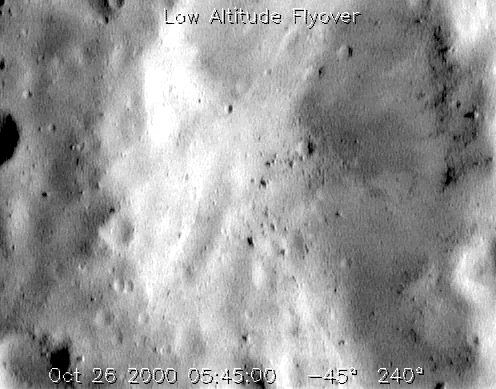
Now, we investigate matching rate of the two approach among real image sequence. Three image sequences that represent different terrain are chosen. The first sequence is shown in Fig. 19. The second sequence were taken at the place that were far from 433 Eros as shown in Fig. 28, the interval between the adjacent images was about 144 s, and the size of each image is 498 × 393, in this sequence, many irregular craters spread on the surface of asteroid, and the illumination change is obvious. The third sequence has 7 images, as shown in Fig. 29, the size of each image is 496 × 389, and the interval between adjacent images was about 75 s. Compare with the first two sequences, they third sequence were taken at a lower height, and the terrain is simple with flat land. For investigate the performance under the situation of large viewpoint changed, the first image is taken to match with the other 6 images respectively in the first two image sequence. For investigate the performance under the situation of obvious span between two images, each image is taken to match with the image that their interval is 1 in the third sequence, for example, 1m3 means the first image matched with the third, and their interval is 1.

Fig. 28

The second image sequence [NASA PHOTO near_descent_157416548 ). a 1; b 2; c 3; d 4; e 5; f 6; g 7

Fig. 29

The third image sequence (NASA PHOTO near_flyover_anim_large). a 1; b 2; c 3; d 4; e 5; f 6; g 7

In general, more feature points can be detected compare with characteristic areas in the same image as described above, so, observe Fig. 30, which illustrates the comparisons of correct matched pairs between SIFT and the approach this paper proposed, therefore, the performance of SIFT is better than the proposed method. However, the gap between SIFT and proposed method became smaller and smaller with the angle of view increased.

Fig. 30

Comparison on the number of correct matched pairs a The first sequence. b The second sequence. c The third sequence

Comparisons of performance on the matching rate is shown in Fig. 31. In the first and second sequence, the matching rate of both method decreased with the interval between matched images increased, although the different between the two methods in the first sequence is not obvious, however, the matching rate of the proposed method can be maintain at a higher level compare with SIFT. The matching rate can maintain the level above 0.2 in the third sequence. So, in the condition of change among image sequence increased, the proposed approach have better robustness compare with SIFT. Figures 32, 33 and 34 illustrate the result with mismatched pairs eliminated by SKINNER-RANSAC.

Fig. 31

Comparison on the matching rate a The first sequence. b The second sequence. c The third sequence

Fig. 32

The matching results with correct matched pairs in the first image sequence. a 1m2; b 1m3; c 1m4; d 1m5; e 1m6; f 1m7

Fig. 33

The matching results in the second image sequence. a 1m3; b 2m4; c 1m4; d 3m5; e 4m6; f 5m7

Fig. 34

The matching results in the third image sequence. a 1m2; b 1m3; c 1m4; d 1m5; e 1m6; f 1m7

Rectification of mismatching pairs is carried out here, it is illustrated in Fig. 35, 36 and 37, from which, all the image pairs have no mismatching pairs. The mismatching pairs are rectified by the method that is proposed in 4.3.

Fig. 35

The results with mismatched pairs rectified in the first image sequence. a 1m2; b 1m3; c 1m4; d 1m5; e 1m6; f 1m7

Fig. 36

The results with mismatched pairs rectified in the second image sequence. a 1m3; b 2m4; c 1m4; d 3m5; e 4m6; f 5m7

Fig. 37

The results with mismatched pairs rectified in the third image sequence

5.2 Experiment on Images with Wide FOV

Most images that are tested above are taken from 433 Eros, and the camera instructed on the detectors had a narrow FOV (Field of View), the focal length is about 167.35 mm, and the FOV is about 2.93° × 2.25°. So, the changes between the consecutive images were not apparent. In this section, images that taken by cameras with wide FOV will be conducted. We have two pairs of images that were taken from Moon to test.

The first pair is a couple of images that were taken in the mission of Apollo 15, as shown in Fig. 38, the images’ height is about 4.5″, the width is about 45.24″, and the focal length is about 609.6 mm, so the FOV is about 10.5° × 85.6°. Observe the images carefully, we can find that the change of illumination is significant obvious. Figure 39 illustrates the matching result with the approach this paper proposed, the number of correct matched pairs is 160, and the number of the total matched pairs is 732.

Fig. 38

The first pair: a couple of images taken from Moon in the mission of Apollo 15 (NASA PHOTO AS15-P-9621, NASA PHOTO AS15-P-9626)

Fig. 39

Matching result in the first pair. a Correct matched pairs extracted; b mismatched pairs rectified

The second pair were taken during Apollo 17. As shown in Fig. 40, the image’s height is about 23 mm, the width is about 35 mm, and the focal length is about 55 mm, so the FOV was about 23.6° × 35.3°. Observe the images, we find that, no matter the illumination or the angle of view between them, the difference was obvious. Figure 41 illustrates the matching result with the method this paper proposed, the number of correct matched pairs is 68, and the total number of matched pairs is 357.

Fig. 40

The second pair: a couple of images taken from Moon in the mission of Apollo 17 [NASA PHOTO AS17-159-23923, NASA PHOTO AS17-159-23924)

Fig. 41

The second pair. a Correct matched pairs extracted; b mismatched pairs rectified

5.3 Consuming time

Processing time of proposed approach will be discussed in this section, the environment of experiment is under MATLAB 2013a, and the operating system is Windows 7. In the Sect. 5.1. As we know that real-time requirement is actually a curtail factor that may decide whether the mission can be achieved successfully in the program of navigation, especially in the autonomous navigation. However, at present, the proposed method suffers the problem of real-time requirement. The average consuming time by the proposed method is about 28–40 s, but the average consuming time by SIFT is about 10–21 s. Therefore, how to reduce the consuming time efficiently can be seen as a mission in the future’s work. We found the step of calculation distance between different shadow areas in the process of processed approach occupied nearly 60% of consuming time, which can be reduced by using K-d tree (Bentley 1975), or making movement estimation in the process of planetary landing, then for each shadow area, just calculate the distance with the areas that may around it.

6 Conclusion

An approach for shadow areas robust matching was proposed for visual automation navigation in planetary landing. Firstly, shadow areas extraction with stable shape based on MSER is introduced in the second section. Secondly, the normalization of shadow areas was introduced in the third section. For better describing the features of normalized shadow areas, a new descriptor named “MA-SIFT” was proposed in this paper, and then compare the descriptor with SIFT and GLOH, we found that the performance of MA-SIFT was better. Thirdly, SKINNER-RANSAC, which is proposed from RANSAC to eliminate the mismatched pairs, and followed by a method of mismatched pairs ‘rectification. Fourthly, several experiments were conducted to compare with SIFT, number of the shadow areas detected is less than the number of feature points detected by SIFT, however, proposed approach has better performance on correct matching rate. At last, images that were taken by cameras with wide FOV were conducted here, the result showed that the proposed method not only can be applied in the images with narrow FOV, but also can be used in the images with wide FOV. However, future work are still needed to be done, they can be concluded as follows:

• 1. The number of the shadow areas detected is less than the number of feature points detected by SIFT, if the terrain is simple, with no craters, rocks and mountainous, that will not suitable to apply the proposed approach.

• 2. Time consuming of the approach doesn’t meet with the requirement of real-time.

• 3. Shadow areas extraction by MSER causes the overlapping among some areas, which may bring the redundant data that cause the waste of time consuming.

References

A. Agarwal, C.V. Jawahar, P.J. Narayanan, A survey of planar homography estimation techniques. Centre for Visual Information Technology, Tech. Rep. IIIT/TR/2005/12 (2005)
A. Ansar, Y. Cheng, Vision technologies for small body proximity operations. I-SAIRAS Conference Proceedings, Sapporo, Japan. 402–409 (2010)
H. Bay, A. Ess, T. Tuytelaars et al., Speeded-up robust features (SURF). Comput. Vis. Image Underst. 110(3), 346–359 (2008)
A. Benedetti, P. Perona, Real-time 2-D feature detection on a reconfigurable computer. Computer Vision and Pattern Recognition, 1998. Proceedings. 1998 IEEE Computer Society Conference on. IEEE, 586–593 (1998)
J.L. Bentley, Multidimensional binary search trees used for associative searching. Commun. ACM 18(9), 509–517 (1975)
J.Y. Bouguet, P. Perona, Visual navigation using a single camera. Computer Vision, 1995. Proceedings. Fifth International Conference on. IEEE, 645–652 (1995)
Y. Cheng, A. Ansar, Landmark based position estimation for pinpoint landing on mars. Robotics and Automation, 2005. ICRA 2005. Proceedings of the 2005 IEEE International Conference on. IEEE, 4470–4475 (2005)
Y. Cheng, A.E. Johnson, L.H. Matthies, et al., Optical landmark detection for spacecraft navigation. Proc. 23th Annual AAS/AIAA Space Flight Mechanics Meeting (2003)
C.D. Epp, T.B. Smith, Autonomous precision landing and hazard detection and avoidance technology (ALHAT), 1–7 (2007)
Eros, The Final Approach. The Johns Hopkins University Applied Physics Laboratory, Laurel, Maryland. http://near.jhuapl.edu/iod/20010731/index.html
M.A. Fischler, R.C. Bolles, Random sample consensus: a paradigm for model fitting with applications to image analysis and automated cartography. Commun. ACM 24(6), 381–395 (1981)
P. Gaudiano, C. Chang. Adaptive obstacle avoidance with a neural network for operant conditioning: experiments with real robots.Computational Intelligence in Robotics and Automation, CIRA’97. Proceedings. 1997 IEEE International Symposium on. p. 13–18 (1997)
C. Harris, M. Stephens, A combined corner and edge detector, vol. 15. Alvey vision conference. (1988), p. 50
A.E. Johnson, H.L. Mathies, Precise image-based motion estimation for autonomous small body exploration. Artificial Intelligence, Robotics and Automation in Space vol. 440. (1999), p. 627
A.E. Johnson, J.F. Montgomery, Overview of terrain relative navigation approaches for precise lunar landing. IEEE Aerospace Conference IEEE, 1–10 (2008)
A.E. Johnson, E. Andrew, et al, Analysis of on-board hazard detection and avoidance for safe lunar landing. 1–9 (2008)
A. Johnson, R. Willson, Y. Cheng et al., Design through operation of an image-based velocity estimation system for Mars landing. Int. J. Comput. Vision 74(3), 319–341 (2007)
Y. Ke, R. Sukthankar, PCA-SIFT, A more distinctive representation for local image descriptors, Vol. 2. Computer Vision and Pattern Recognition, 2004. CVPR 2004. Proceedings of the 2004 IEEE Computer Society Conference on. IEEE, 2: II-506-II-513 (2004)
D.G. Lowe, Distinctive image features from scale-invariant key points. Int. J. Comput. Vision 60(2), 91–110 (2004)
W. Lu, H. Lu, F.L. Chung, Feature based robust watermarking using image normalization. Comput. Electr. Eng. 36(1), 2–18 (2010)
J. Matas, O. Chum, M. Urban et al., Robust wide-baseline stereo from maximally stable extremal regions. Image Vis. Comput. 22(10), 761–767 (2004)
J.F. Montgomery, A.E. Johnson, S.I. Roumeliotis et al., The jet propulsion laboratory autonomous helicopter tested: a platform for planetary exploration technology research and development. J. Field Robot. 23(3–4), 245–267 (2006)
J.J. Moré, The Levenberg-Marquardt algorithm: implementation and theory. Lecture Notes in Mathematics 630, 105–116 (1978)
P. Moreno, J. Bernardin, J. Santos-Victor, Improving the SIFT descriptor with smooth derivative filters. Pattern Recogn. Lett. 30(1), 18–26 (2009)
NASA PHOTO near_20000919_large_anim: http://nssdc.gsfc.nasa.gov/planetary/image/near_20000919_large_anim.gif
NASA PHOTO near_20000511:http://nssdc.gsfc.nasa.gov/planetary/image/near_20000511.jpg
NASA PHOTO near_flyover_anim_large: http://nssdc.gsfc.nasa.gov/planetary/image/near_flyover_anim_large.gif
NASA PHOTO near_descent_157416548: http://nssdc.gsfc.nasa.gov/planetary/image/near_descent_157416548.jpg
NASA PHOTO near_descent_157415118: http://nssdc.gsfc.nasa.gov/planetary/image/near_descent_157415118.jpg
NASA PHOTO AS15-P-9621: http://www.lpi.usra.edu/resources/apollo/frame/?AS15-P-9621
NASA PHOTO AS15-P-9626: http://www.lpi.usra.edu/resources/apollo/frame/?AS15-P-9626
NASA PHOTO AS17-159-23923: http://www.lpi.usra.edu/resources/apollo/frame/?AS17-159-23923
NASA PHOTO AS17-159-23924: http://www.lpi.usra.edu/resources/apollo/frame/?AS17-159-23924
N. Ohtsu, A threshold selection method from gray-level histograms. IEEE Trans. Syst. Man Cybern. 9(1), 62–66 (1979)
S.C. Pei, C.N. Lin, Image normalization for pattern recognition. Image Vis. Comput. 13(10), 711–723 (1995)
B.V. Pham, S. Lacroix, M. Devy, et al., Landmark constellation matching for planetary lander absolute localization. Visapp 2010—Proceedings of the Fifth International Conference on Computer Vision Theory and Applications, Angers, France: 267–274 (2010)
B.V. Pham, S. Lacroix, M. Devy et al., Fusion of absolute vision-based localization and visual odometry for spacecraft pinpoint landing. Prague Cz (2010)
C. Schmid, R. Mohr, Local gray value invariants for image retrieval. IEEE Trans. Pattern Anal. Mach. Intell. 19(5), 530–535 (1997)
J. Shi, C. Tomasi, Good features to track. Computer Vision and Pattern Recognition, 1994. Proceedings CVPR’94. 1994 IEEE Computer Society Conference on. IEEE, 593–600 (1994)
B.F. Skinner, The behavior of organisms (Appleton Century Crofts, New York, 1938), p. 110–150
N. Trawny, A.I. Mourikis, S.I. Roumeliotis, et al., Coupled vision and inertial navigation for pin-point landing. NASA Science and Technology Conference (2007)
P.G. Wetzler, R. Honda, B. Enke, et al., Learning to detect small impact craters. Application of Computer Vision. WACV/MOTIONS’05 Volume 1. Seventh IEEE Workshops on. IEEE, 1, 178–184 (2005)
M. Yu, H. Cui, Y. Tian, A new approach based on crater detection and matching for visual navigation in planetary landing. Adv. Space Res. 53(12), 1810–1821 (2014)
Acknowledgements
Colleges and Universities in Hebei Province Science and Technology Research Project (No. QN2016223); 2016 Hebei University of Economics and Business, Dr. Scientific Research Fund (No. 0112160171); 2016 Hebei University of Economics and Business, Research Fund (No. 2016KYQ01); National Natural Science Foundation of China (No. 61375086); National Basic Research Program of China (973 Program) (No. 2012CB720000).We thank the above mentioned funds for the financial support.
Author information
Authors and Affiliations
Corresponding author
Rights and permissions
About this article
Cite this article
Ruoyan, W., Xiaogang, R., Naigong, Y. et al. Shadow Areas Robust Matching Among Image Sequence in Planetary Landing. Earth Moon Planets 119, 95–124 (2017). https://doi.org/10.1007/s11038-016-9502-5
Received:
Accepted:
Published:
Issue Date:
DOI: https://doi.org/10.1007/s11038-016-9502-5