
Abstract
Ten small rock slides (with a volume ranging from 101 to 103 m3) on a slope affected by working activities were detected, located, and timed using pictures collected by an automatic camera during 40 months of continuous monitoring with terrestrial SAR interferometry (TInSAR). These landslides were analyzed in detail by examining their pre-failure time series of displacement inferred from high-sampling frequency (approximately 5 min) TInSAR monitoring. In most of these cases, a typical creep behavior was observed with the displacement starting 370 to 12 h before the collapse. Additionally, an evident acceleration decrease of the displacement a few hours before the failure was observed in some rock/debris slides, thus suggesting the possibility of a mechanical feature of the slope that differs from the classical creep theory. The efficacy of the linear Fukuzono approach for the prediction of time of failure was tested by back-analyzing the ten landslides. Furthermore, a modified Fukuzono approach named average data Fukuzono (ADF) was implemented and applied to our dataset. Such an approach is able to improve forecasting effectiveness by reducing the error due to anomalies in the time series of displacement, like the acceleration decrease before failure. A prediction with a temporal accuracy of at least 2 h was obtained for all the analyzed rock/debris slides.
Introduction
Landslide prediction is a major step toward reducing the impact of natural disasters and risks related to human activities in mountainous and hilly areas. Landslides are complex natural phenomena involving volumes ranging from some cubic meters up to some hundreds of millions of cubic meters. Landslides do not behave as a perfectly rigid and brittle body; hence, they are always affected by deformation before the failure (Siddle et al. 2007). The trend of deformation vs. time is considered one key factor in allowing the prediction of time of failure. The amount of pre-failure deformation spans several orders of magnitude (from a few millimeters to several meters) depending on the type of material involved in the landslide, the slope geometry, and the landslide trigger. However, landslides are often characterized by a complex geometry and a combination of heterogeneous materials with different features, thus leading to a nonlinear behavior before the failure. Temporal variation of preconditioning and triggering factors such as climate, river activity, tectonics, and human activities further complicate the evolution of landslides over time.
Since the 1960s, several studies have been carried out with the aim to define rules and procedures to estimate the time of failure of landslides (i.e., Saito 1965; Fukuzono 1990; Voight 1988; Crosta and Agliardi 2002). Semi-empirical approaches based on the analysis of displacement (or derived values) time series have been developed and tested on both laboratory-scale and real events, sometimes obtaining good results in terms of landslide forecasting. All these approaches require the collection of displacement data before the failure by a suitable displacement monitoring technique. Back-analysis of large landslides, e.g., the 1963 Vajont landslide (Kilburn and Petley 2003), has demonstrated the efficacy of these approaches in predicting past landslides, but it also highlights the difficulties in predicting the failure time of present landslides (Crosta and Agliardi 2003). All these past studies suffer from the great complexity and infinite variety of landslides from the low quality of displacement data available in terms of temporal resolution in data collection, accuracy, and spatial resolution. In fact, the most recent studies still employ point-based techniques (e.g., inclinometers, extensometers) or monitoring systems with a low temporal frequency in data collection (days to hours) or low accuracy in displacement measurement, etc. In other words, little attention has been given to the importance of monitoring data and to related monitoring methods (Dunnicliff 1988) to improve the forecasting efficacy, even if over the last few years innovative and advanced monitoring techniques have been developed, especially in the remote sensing field (Mazzanti 2012).
Terrestrial SAR interferometry (TInSAR) (Mazzanti 2011; Luzi 2010), also known as ground-based SAR interferometry (GBInSAR), is one of the most recent and most powerful of these techniques for monitoring landslides. This technique has the following main advantages: (1) fully remote monitoring (no installation in dangerous areas is required); (2) widespread monitoring instead of the monitoring of single points; (3) simultaneous monitoring of a high number of points (up to hundreds of thousands); (4) high accuracy in surface displacement monitoring (up to decimal millimeters); and (5) a high data sampling rate (up to a few seconds). These improved capabilities play a fundamental role in the attempt to predict the time of landslide failures, thus allowing, for example, identification of the precise area affected by the movement (widespread view), cross-validation of the displacement time series by the enormous number of monitoring points, and the acquisition of dense and accurate time series.
A field experiment was carried out to evaluate the new opportunities offered by the TInSAR monitoring data for time of failure prediction purposes. Four years of continuous monitoring of an unstable slope by TInSAR with a data sampling rate of 5 min allowed the study of the pre-failure behavior of ten small-scale landslides identified on optical images. The relevant improvements in the forecasting methods for landslide time of failure are also investigated in detail.
Landslide failure prediction by displacement time series
The first attempts to predict the time of failure of unstable slopes on the basis of displacement time evolution date back to the early 1960s (Saito and Uezawa 1961; Saito 1965, 1969). By analyzing the rupture of 80 samples on triaxial compression lab tests, Saito observed that displacement was the most useful parameter to predict the time of failure. Hence, Saito (1965) developed a method based on the “slope creep” theory (Terzaghi 1950; Haefeli 1953) to obtain the time before failure using slope displacement data. The creep process is a time-dependent deformation of materials under the action of stresses (e.g., gravity) and is usually divided into three main phases: primary, secondary, and tertiary creep. The failure of materials and slopes usually occurs in the tertiary creep. Therefore, Saito (1969) modified the method to fit nonsteady behavior of landslides in the tertiary creep prior to failure. In the 1980s, improvements to Saito’s prediction model were made by Fukuzono (1985) and Voight (1988, 1989a). Fukuzono showed that the logarithm of velocity of the surface displacement is proportional to the logarithm of the acceleration. In other words, under invariant loading conditions, pre-failure behavior can be described by a power law equation in the following form:
where x is the downward surface displacement along the slope, t is the time, and a and α are dimensionless constant parameters.
According to the results of the experiments by Fukuzono (1985, 1989) and the studies of Varnes (1983) and Yoshida and Yachi (1984), α commonly varies within a range of 1.5–2.2. Therefore, the following equation has been suggested to predict the time of failure:
where v is the surface displacement velocity and t f is the failure time. For α = 2, the resulting curve is linear; for α >2, it is convex; and for 1> α <2, it is concave (Fukuzono 1985). Hence, in the case of α = 2, the failure time can be simply computed by the following equation:
and the time of failure corresponds to the interception of the x-axis of the interpolated straight line in the diagram’s inverse velocity vs. time (Fukuzono 1985).
A more generalized relationship to describe rate-dependent material failure was given by Voight (1988):
where and \( \ddot{\varOmega} \) and \( \dot{\varOmega} \) are the acceleration and velocity of the displacement, respectively.
In terms of time of failure prediction, the following equation can be obtained by assuming \( \dot{\varOmega} \) f (velocity at t f) = infinite:
This assumption leads to nonconservative forecasts, but the error is often small and may not be important to decision makers (Voight 1988).
The efficacy of this method in predicting landslide time of failure has been demonstrated by several authors, including Voight and Kennedy (1979), Voight (1989b), Cornelius and Voight (1990, 1994, 1995), Voight and Cornelius (1990, 1991), Rose and Hungr (2007), and Gigli et al. (2011).
Landslide monitoring by terrestrial SAR interferometry
Continuous monitoring is a key requirement for the prediction of a landslide. Failure prediction can be based on the monitoring of landslide-triggering factors (e.g., rainfall, groundwater level) or of landslide effects (e.g., ground displacement). Over the years, it has been demonstrated that the monitoring of landslide effects is the most effective solution for the control and prediction of landslides. Hence, several technical solutions for the monitoring of ground displacement are currently available. These techniques can be divided into two main categories:
-
Geotechnical contact techniques, including extensometers, inclinometers, and strainmeters (see Dunnicliff (1988) for an extensive review)
-
Remote techniques, including topographic systems, photogrammetry, laser scanning and SAR Interferometry (see Mazzanti (2012) for an extensive review)
Of these techniques, differential SAR interferometry (DInSAR) is among the newest and most powerful, and its features fit well with landslide monitoring requirements. DInSAR was developed for satellite applications in the early 1990s and was originally used to measure ground displacements at a regional scale (Curlander and McDonough 1991; Massonet and Fiegl 1998; Hanssen 2001). In the late 1990s and early 2000s, several innovation occurred in the SAR field such as the development of innovative approaches for satellite data processing based on data stacking (Ferretti et al. 2001) and the development of the first ground-based SAR equipment prototypes. Over the last 10 years, both satellite and terrestrial InSAR have been extensively used for landslide monitoring, thus demonstrating their efficacy (Pieraccini et al. 2002; Leva et al. 2003; Tarchi et al. 2003; Antonello et al. 2004; Hilley et al. 2004; Strozzi et al. 2005; Noferini et al. 2005; Casagli et al. 2006; Colesanti and Wasowski 2006; Farina et al. 2006; Herrera et al. 2009; Bozzano et al. 2010; Intrieri et al. 2012).
The TInSAR technique is based on an active radar sensor that emits microwaves and receives the return of scattering objects. In the most common configuration, the sensor, which has two antennas (one emitting and one receiving), moves along a linear rail, thus collecting an enormous number of radar images with a single resolution (range resolution). Then, by combining images collected during a single scan through the synthetic aperture radar principle, bidimensional images are derived, thus introducing the cross-range resolution (Fig. 1). The ground cross-range resolution can be approximated as

Example of grid resolution
where Δa is the cross-range resolution, r is the range distance (i.e., the distance between the GB-SAR system and the measured point), λ is the central wavelength, and L is the length of the rail.
This means that considering a wavelength of approximately 17 mm and a rail length of 2 m (the features of the equipment used in this paper), the cross-range resolution is on the order of 0.4 and 4 m at a distance of 100 and 1,000 m, respectively.
For the range resolution, the equipment used in this study is based on the stepped frequency-continuous wave (SF-CW) principle, in which a band of continuous electromagnetic waves having different frequencies are emitted. The range resolution is equal to:
where c is the light velocity and B is the radiofrequency bandwidth. By Eq. 7, we can observe that the range resolution is constant (i.e., it is independent of the range distance) and that it only depends on the bandwidth. For example, with a bandwidth of 200 MHz, the maximum range resolution is on the order of 0.75 m.
The final result of TInSAR data acquisition is a bidimensional image made of pixels (up to some millions), whose footprint size increases with increasing instrument target distance.
Each pixel of the image is featured by a complex number, namely amplitude and phase values that are specific for a certain polarization, electromagnetic frequency, and incidence angle (Ulaby et al. 1982).
The signal to noise ratio (SNR) value is one of the parameters for assessing the backscattering features of a specific target (i.e., localized area) inside the investigated scenario. Both mean values or variability over time of this value on data stack are used.
The phase at each pixel can be used for the estimation of displacement through the interferometric technique. In other words, the phase difference of each pixel of two or more SAR images collected at different times is computed and, in the case of long stacks of images, cumulated over time. In terrestrial SAR interferometry, the computed phase difference (Δφ) is mainly controlled by the following factors:
where Δφ displ is the phase shift contribution due to the ground displacement, Δφ atmos is the phase shift contribution due to the atmospheric changes, and Δφ noise is the phase shift contribution due to the instrumental noise. By assuming that the Δφ noise is random and not relevant, once the Δφ atmos is computed, the Δφ displ can be derived. Therefore, the displacement is computed by the following equation:
where d is the displacement computed along the line of sight (LOS), λ is the wavelength of the radar signal, and Δφ is the phase difference between the two acquisitions.
Hence, the accuracy in the displacement measurement depends on the signal’s wavelength, the atmospheric conditions, and the sensing distance. Specifically, the lesser the distance and the more stable the atmospheric conditions, the higher the accuracy of the displacement measurements (from 0.01 mm in the lab to a few millimeters in the field).
It is worth noting that the interferometric analysis implies some limitations concerning the displacement measurement due to the cyclic behavior of the phase. As a matter of fact, the phase unwrapping (e.g., Goldstein et al. 1988) is a key part of the interferometric analysis for displacement measurement. Considering the wavelength of the herein used GBSAR equipment, the phase ambiguity is on the order of 4.5 mm (i.e., the λ/4 value) that can be assumed as 9 mm if we assume that inversion of displacement direction along the line of sight cannot occur.
The coherence value, which evaluates the correlation among the phases at each pixel, is a good estimator of the phase stability and, therefore, can be used for a preliminary evaluation of the expected displacement accuracy. This value ranges between 0 and 1, where 0 is the complete decorrelation of the phase and 1 is the complete correlation (Hanssen 2001). Hence, multitemporal analysis allows LOS displacement time histories of each pixel of the image to be obtained (Bozzano et al. 2011).
In summary, the following operational features make the TInSAR technique particularly suitable for the monitoring of landslides and for failure forecasting: (1) the ability to yield data and answers within a brief time (a few minutes); (2) efficacy under any weather and lighting conditions; (3) completely remote operability (it does not require the installation of sensors or targets on the monitored slope); (4) continuous distributed monitoring of the entire slope with a high pixel resolution; and (5) long-range monitoring (up to some kilometers).
Notwithstanding the numerous TInSAR successfully applications cited above, little attention has been devoted to the opportunities offered by this technique for landslide prediction purposes and still less for small-scale landslides.
The study area
The field experiment presented herein concerns a slope affected by a major deep-seated landslide characterized by a very complex geological and geomorphological setting (Bozzano et al. 2008, 2011). Due to the development of a major communication road, the slope has been extensively investigated since 2007 and controlled for more than 4 years by an integrated monitoring platform composed of traditional sensors (inclinometers, piezometers, load cells, and topographic measures) and a remote station equipped with an IBIS-L terrestrial SAR interferometer, by IDS S.p.A (Table 1), a weather station, and an automatic camera. These equipment was housed in a specially designed box and installed on the opposite slope to the one involved in the project, at a distance ranging from 700 to 900 m (Fig. 2). The remote monitoring network has been active 24/7 from November 2007 until now. Collecting TInSAR data at a sampling rate of approximately 5 min, the network has thus far collected more than 20,000 pictures, 400,000 measurements of weather data, and 400,000 SAR images (Bozzano et al. 2011). The digital camera and the weather station, featuring an automatic data acquisition and transfer system, have played a key role in the monitoring activity. The images continuously supplied by the camera have made it possible to continuously monitor the construction activities and the engineering works on the investigated slope, thereby optimizing data collection and processing. This functionality also facilitates the interpretation of the results and the optical first identification and timing of landslides. In fact, during the experimental period, the slope was frequently affected by shallow translational landslides (with a volume ranging from 101 to 104 m3), which represent surface evidence of a deep landslide (Bozzano et al. 2011). These landslides were identified and located by optical photos (Figs. 3 and 4) and then detailed in terms of location over the slope and time of occurrence by TInSAR displacement images. Detailed and accurate SAR displacement images and cumulative time series of each pixel inside the landslide area were derived for each landslide.

Sketch showing the monitoring geometry

a, b Pictures before and after landslide 1 (red circle); c, d TInSAR displacement images before and after the landslide overlain on the picture (a, b)

Picture of the slope showing the location of the ten shallow landslides described in Table 2
These landslides were investigated in detail by examining their size and geometry, geological material, and location (Table 2). The landslide volumes range from 101 to 5 × 10² m3, with an estimated maximum thickness of approximately 3 m. The landslides were classified as translational and roto-translational movements involving weathered and fractured gneiss widely outcropping over the slope. These landslides were mainly triggered by rainfall. Some of these landslides occurred in portions of the slope covered by spritz beton. It is worth noting that the sizes of some of the landslides reported in Table 2 are similar to those of the experimental landslides described in the papers by Fukuzono (1990) and Moriwaki et al. (2004).
Pre-failure behavior of small-scale landslides detected by continuous TInSAR monitoring
The displacement behavior of the ten shallow landslides described above, especially at their pre-failure stage, were analyzed in detail to infer information about the total amount of displacement, the duration of the entire process, the velocity, the acceleration, and other factors (Table 3).
For each landslide, we computed the time series of displacement of those pixels that were considered the most representative of the overall landslide behavior. Specifically, pixels were chosen on the basis of the following criteria: (1) the highest quality TInSAR data available on the basis of SNR and coherence analysis; (2) pixels clearly located within the main landslide body (and not in the surrounding parts affected by tensional release); and (3) pixels located preferably in the topographic upper part of the landslides, as they are assumed to be less influenced by internal deformation.
Thanks to the high temporal information density (one displacement value every about 5 min), it was possible to process the identified time series using a digital filter to remove the noise. A direct-form FIR equiripple lowpass filter, implemented in the “filtfilt” algorithm (Matlab 7), was used for the filtering, thus significantly improving the quality of the time series (Fig. 5). Data filtering is very important for our purposes, as the used models for landslide prediction are based on landslide velocity, i.e., the displacement noise is commonly amplified.

a Displacement time series and filtered displacement time series; b applied direct-form FIR Equiripple lowpass filter: D pass and D stop = passband and stopband ripples; ω pass and ω stop = transition width
Once achieved, the final time series landslides were analyzed, thus deriving the following:
-
1.
The temporal evolution of displacement, i.e., the initiation of the movement (manually identified on the time series as the intersection point between horizontal trend lines and a clearly detectable inclined trend lines when a cumulative displacement of 2 mm is achieved), and the final collapse of each landslide were exactly dated and timed with a precision of a few minutes, thus obtaining values ranging from a couple of weeks to a few hours (Fig. 6).
Fig. 6 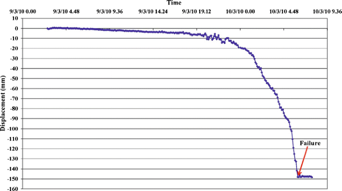
Example of time series of displacement derived from TInSAR monitoring data (landslide n.10). The failure time can be clearly identified with a precision of a few minutes thanks to the sudden stop in the displacement
-
2.
The total landslide displacement from its onset to its collapse, thus achieving values ranging from a couple of centimeters up to 1 m (Fig. 7).
-
3.
Maximum velocity, thus achieving values ranging from 8 to 64 mm/h (Fig. 8).


It is worth noting that all the landslides, apart from 2, 4, and 8, were characterized by the maximum velocity just before the collapse, thus showing a trend of velocity continuously increasing since the landslide start until the failure. The peak of acceleration was registered in all the landslides some hours before the collapse instead (Fig. 8).
In other words, the final stage of the landslide displacement was characterized by an increasing velocity but a decreasing acceleration rate. The peak acceleration of the landslides ranged from 1 to 82 mm/h2, depending on the landslide. The value of acceleration decrease (computed as the difference between the peak acceleration and the last value available before the failure) ranged from 2 to 154 mm/h2. Furthermore, the value of acceleration decrease is closely proportional to the peak acceleration value of the landslides. Specifically, the ratio between the value of acceleration decrease and the acceleration peak ranges from 0.8 to 2.1. It is worth noting that the achieved values of total displacement, velocity, and acceleration were very similar to those measured in the experiments by Fukuzono (1985) and Moriwaki et al. (2004), which is a further confirmation of the quality of the dataset presented herein, which is comparable to the data derived from a controlled experiment.
Nevertheless, it is worth noting that pre-failure acceleration decrease is something never observed before, whether in field or experimental landslides. This evidence, which could play a relevant role in time of failure prediction, was obtained thanks to the availability of accurate and high-sampling rate data.
Time of failure analysis of detected landslides
The large dataset of events occurred on the same slope (which means similar conditions and features of the landslides), and the detailed displacement data available represent a rare occasion to test the efficacy of semi-empirical approaches based on time series of displacements (or derived quantities such as velocity and acceleration). Furthermore, to the authors’ knowledge, semi-empirical approaches have previously been tested mainly on large-scale real landslides, except for the large-scale experiments by Fukuzono (1985) and Moriwaki et al. (2004). Hence, the presented dataset is quite new in this field of research.
In this paper, analyses based on the simple linear Fukuzono (α = 2) approach are presented (as it is the most commonly used for time of failure prediction purposes) to infer their efficacy in predicting the time of failure of the landslides investigated herein. For each landslide, the predicted time of failure was computed iteratively since the beginning of the displacement phase (looking at the tertiary creep phase) by increasing the number of displacement data step by step. Hence, the real prediction of the time of failure based on the newly collected data over time was computed. In other words, the dataset used for the computation of the time of failure is progressively enlarging with time, and consequently, the prediction is updated. For each landslide, the obtained results were plotted in a diagram showing the predicted time of failure in the x-axis and the time of elaboration before failure (in hours) in the y-right axis (blue line in Fig. 9). For example, 1.6 h before failure, the predicted time of failure of landslide 3 computed by using the time series of displacement allowable until this time was 14:42 instead of 15:36 (red line in Fig. 9) as what really occurred. In contrast, 0.1 h before failure, the time of failure of landslide 3 was exactly predicted. Starting elaboration time (yellow line in Fig. 9) was roughly identified on the time series of displacement by using a graphical method similar to that one used in soil mechanics to identify yield stress on the stress-strain odometric curve.

Diagram showing the variation of the time of failure prediction using an incremental dataset length for landslide 3. Green line is the “time series of displacement” (left y-axis vs. time in abscissa); blue line is the updating of the prediction during the 2 h before the failure (right y-axis vs. time of failure in abscissa). Recorded time of failure is marked by the red line; yellow line is the starting time for the computation
Diagrams showing the temporal discrepancy between the real and predicted time of failure over time (e.g., the quality of prediction over time) were obtained for the ten landslides (Fig. 10).

Three hours is the maximum absolute error in the landslide time of failure prediction except for landslides 2 and 9 (Figs. 4 and 11 and Tables 2 and 3). In these two cases, the maximum error was on the order of 600 to 1,000 h, i.e., longer than the entire timespan of the landslide. Landslides 2 and 9 were characterized by longer time series of displacement and by a spurious creep behavior characterized by several acceleration increase and decrease phases before the failure. Such a pattern of displacement can be considered the main reason for the low performances of the linear Fukuzono analysis.

a–f From left to right (upper and lower diagrams), the results of the Fukuzono analysis using the conventional approach, the average approach, and the moving average approach for landslide 2
For the other eight remaining landslides, the error in the predicted time of failure is very small. Specifically, for five landslides (1, 3, 6, 8, and 10), positive prediction error was found (i.e., predicted time of failure postponed with respect to the real landslide occurrence), while for two landslides (4 and 7), negative error (i.e., predicted time of failure anticipated respect to the real one) was found. Our attention was mainly concentrated on the positive errors as they are contrary to general precautionary principles.
To ameliorate these problems, a new approach named average data Fukuzono (ADF) was developed. ADF is a modified version of the Fukuzono method consisting of the average and moving average velocity computed from temporal consecutive data. In the first case, the data were averaged iteratively, starting from the first data collected. In the case of the moving average, the data were averaged by using half of the dataset moved iteratively by one single step until the last half before the failure.
Figure 11 shows the results achieved using the ADF approach for landslide 2. As can be seen, both the average and the moving average approaches (Fig. 11b, c, e, f) significantly reduce the prediction error achieved by using the standard Fukuzono method and reported in Fig. 11a, d.
Figure 12 shows the results achieved by using the ADF approach for landslide 10. In this case, the error obtained by the standard Fukuzono analysis (Fig. 12a, d) is quite small; hence, the quality of the prediction is only slightly improved by the ADF approach (Fig. 12b, c, e, f). However, the moving average significantly reduces the error in the final phase of displacement, thus avoiding the negative effect due to the decelerating phase.

a–f From left to right (upper and lower diagrams), the results of the Fukuzono analysis using the conventional approach, the average approach, and the moving average approach for landslide 10
The efficacy of the ADF approach in reducing the positive prediction errors is clearly visualized in Fig. 13, where the mean value of the prediction error and the related standard deviation of the dataset of the five landslides are shown by normalizing the time.

Comparison between the error of the prediction of the failure time for landslides 1, 3, 6, 8, and 10 by using the linear Fukuzono method and the moving average ADF method. Time in abscissa is normalized with respect to the time of failure of each five landslides and error at each normalized time step is the mean error value for the five landslides; bars are referred to the standard deviation associated to the mean value at each time step
Discussion
A long-term continuous monitoring of the displacement of an unstable slope (whose size is on the order of 0.2 km2) by TInSAR allowed us to build a spatio-temporally high-resolution dataset describing the pre-failure behavior of minor small and shallow landslides (a few tenths of cubic meters) with an accuracy of 1 mm. Some of these landslides were similar in size to the experimental ones proposed by Fukuzono (1985) and Moriwaki et al. (2004) and were characterized by similar displacement behavior before failure (in terms of total displacement, velocity, and acceleration values). However, while the abovementioned experiments were performed on a single “ideal” landslide (whose features were previously defined), our dataset was made of ten landslides that occurred in a field environment. Continuous monitoring by terrestrial SAR interferometry provided an unquestionable contribution to this study, thus allowing us to achieve data as of high quality as can be achieved on a lab experiment. Specifically,
-
1.
The high temporal resolution (about 5 min) on data collection allowed us to characterize also the displacement of landslides that occurred in a short time span (few hours) with a high data sampling rate, thus allowing us to identify the last steps of the creep process before failure.
-
2.
The spatially continuous monitoring (i.e., displacement maps instead of single points) with a high ground resolution (few meters) allowed us to measure the displacement also of small landslides (few tenths of square meters) and, in some cases, to cross-check the inferred displacement from adjacent pixels.
-
3.
The high accuracy in the displacement measurement allowed us both to characterize landslides with a small pre-failure displacement (even a couple of centimeters) and to well define their acceleration behavior.
-
4.
The capability of TInSAR to collect data under any weather and lighting conditions allowed us to get information about events that occurred on complex environmental conditions and during the night.
Furthermore, it is worth stressing that the opportunity of monitoring an entire slope with a high spatial continuity was a key feature that allowed us to detect and characterize landslides that occurred also in sectors that were not originally planned.
Nevertheless, it is important to account also for some of the limitations of terrestrial InSAR monitoring and on their effects on the results achieved in this study:
-
1.
First of all, as TInSAR provides only surface displacement data, no information was available on the deep behavior of the investigated landslides. However, considering the shallow feature of the herein discussed landslides, such a limitation is not considered relevant for this study.
-
2.
Phase ambiguity problem, especially in the final evolution phases before the failure when the displacement velocities are higher. As a matter of fact, considering the usual small size of the landslides, spatial unwrapping algorithms demonstrated to be not very effective and only a temporal phase unwrapping was used, supported by the authors’ expertise in the TInSAR data processing. In this regard, it is worth noting that, for most of the landslides, the velocity in the final stage is well below the phase ambiguity threshold (4.5 or 9 mm in 5 min, if we assume that inversion of direction of movement is not reasonable for a landslide), and it is more than reasonable to assume that the phase ambiguity problems have not happened. However, in some cases (such as numbers 4, 9, and 10), this occurrence cannot be excluded. Furthermore, no other data derived from different sensors have been collected.
Anyway, instead of what was stated above, all these landslides were characterized by a similar displacement pattern in terms of peak values of velocity and acceleration and time-dependent evolution. However, a peculiar acceleration decrease before failure was observed in several landslides in our dataset. Such a behavior represents an anomaly with respect to available data from the literature and, at present, cannot be explained by existing theoretical creep models that assume a continuous increasing of acceleration until failure. This pre-failure acceleration decrease has several implications in the application of the already-existing semi-empirical models based on the creep theory, as demonstrated by the analyses performed by the simple linear Fukuzono approach (Fig. 9). The pre-failure acceleration decrease leads to a delay in the failure time with respect to that previously predicted by using the linear Fukuzono approach. Such behavior cannot be fully understood by the available data, and it requires further study. Nevertheless, we cannot neglect that the creep theory assumes a deformation under the condition of constant stress. Such a condition is not considered in our experiments because rainfall occurred during the experiments; hence, we cannot exclude the possibility that this condition could be one of the reasons for the pre-failure acceleration decrease. However, it is worth noting that the constant strain condition is also not considered in actual large landslides, such as those studied by Crosta and Agliardi (2003). The effect of rainfall was observed in landslides 2 and 9, where multiple acceleration and acceleration decrease phases occurred before the failure. In fact, these landslides are characterized by a high prediction error using the linear Fukuzono approach. The other landslides are always predicted with an error lower than 3.5 h. A drastic reduction in the forecasting errors was achieved by the herein proposed average data Fukuzono (ADF) approach (Fig. 10). This method, which consists of the average and moving average of the displacement data over time, is very effective at reducing the forecasting error, especially for unsteady cases characterized by important decelerating phases (Fig. 11). Furthermore, the ADF approach seems to be very effective in reducing the effect of the final decelerating phase (Fig. 13).
However, it is worth noting that the ADF approach is very sensitive to the number of available data, i.e., detailed time series significantly increase its efficacy, thus confirming the importance of high-resolution monitoring data for landslide prediction.
Conclusions
With the aim of deepening our understanding of landslide pre-failure behavior and, therefore, landslide prediction capabilities, a long-term field experiment using TInSAR was carried out. By analyzing the pre-failure behavior of ten landslides that occurred during the experiment, we showed that high-accuracy and high-sampling rate (a few minutes) of surface displacement data can be successfully used to obtain a good prediction of a landslide’s time of failure. Furthermore, the widespread and high-resolution information retrieved by TInSAR displacement images allows investigation from a remote position and the assessment of the pre-failure behavior of small landslides. In fact, traditional contact monitoring methods may fail due to a low data sampling rate, low accuracy and, particularly, punctual and localized information that may lead to a lack of information or to misinterpretations, especially for small-sized landslides.
A landslide is a very complex process characterized by an infinite range of variable features. The ability to obtain detailed and accurate information about the behavior of landslides is crucial to predict their future evolution (i.e., failure). Existing semi-empirical models based on the creep theory are very effective at predicting time of failure in laboratory experiments, but they are effective for real landslides only in a few cases. However, we demonstrated that by using accurate and high-sampling rate data, these models may be effectively used in real practice. Furthermore, a high data sampling rate allows the effective use of the ADF approach, which is able to drastically improve the efficacy of creep-based prediction methods in the case of “unsteady landslides.” Hence, it can be said that by using TInSAR continuous monitoring and advanced data processing solution such as the ADF approach, we can achieve the same results previously achieved for “ideal” laboratory landslides for real field landslides.
References
Antonello G, Casagli N, Farina P, Leva D, Nico G, Siebar AJ, Tarchi D (2004) Ground-based SAR interferometry for monitoring mass movements. Landslides 1:21–28
Bozzano F, Mazzanti P, Prestininzi A (2008) A radar platform for continuous monitoring of a landslide interacting with an under-construction infrastructure. Ital J Eng Geol Environ 2:35–50
Bozzano F, Mazzanti P, Prestininzi A, Scarascia Mugnozza G (2010) Research and development of advanced technologies for landslide hazard analysis in Italy. Landslides 7(3):381–385
Bozzano F, Cipriani I, Mazzanti P, Prestininzi A (2011) Displacement patterns of a landslide affected by human activities: insights from ground-based InSAR monitoring. Nat Hazards 59(3):1377–1396. doi:10.007/s11069-011-9840-6
Casagli N, Farina P, Leva D, Tarchi D (2006) Application of ground based radar interferometry to monitor an active rockslide and implication for emergency management. In: Evans SG et al (eds) Landslide from massive rock slope failure. Springer, Dordrecht, pp 157–173
Colesanti C, Wasowski J (2006) Investigating landslides with space-borne Synthetic Aperture Radar (SAR) interferometry. Eng Geol 88:173–199
Cornelius RR, Voight B (1990) Feasibility of material failure approach to eruption prediction for Mount St. Helens, 1985 and 1986. EOS Trans Am Geophys Union 71:1693
Cornelius RR, Voight B (1994) Seismological aspects of the 1989–1990 eruption at Redoubt Volcano, Alaska: the materials failure forecast method (FFM) with RSAM and SSAM seismic data. J Volcanol Geotherm Res 62:469–498
Cornelius RR, Voight B (1995) Graphical and PC-software analysis of volcano eruption precursors according to the materials failure forecast method (FFM). J Volcanol Geotherm Res 64:295–320
Crosta GB, Agliardi F (2002) How to obtain alert velocity thresholds for large rockslides. Phys Chem Earth 27(36):1557–1565
Crosta GB, Agliardi F (2003) Failure forecast for large rock slides by surface displacement measurements. Can Geotech J 40:176–191
Curlander JC, McDonough RN (1991) Synthetic aperture radar systems and signal processing. Wiley, New York
Dunnicliff CJ (1988) Geotechnical instrumentation for monitoring field performance. Wiley, New York
Farina P, Colombo D, Fumagalli A, Marks F, Moretti S (2006) Permanent scatterers for landslide investigations: outcomes from the ESA-SLAM project. Eng Geol 88:200–217
Ferretti A, Prati C, Rocca F (2001) Permanent scatterers in SAR interferometry. IEEE Trans Geosci Remote Sens 39:8–20
Fukuzono T (1985) A new method for predicting the failure time of a slope. Proceedings of the fourth international conference and field workshop on landslides, Tokyo, Japan. Landslide Soc 145–150
Fukuzono T (1989) A simple method for predicting the failure time of slope—using reciprocal of velocity, Technology for Disaster Prevention, Science and Technology Agency, Japan. Int Coop Agency, Japan 1(13):111–128
Fukuzono T (1990) Recent studies on time prediction of slope failure. Landslide News 4:9–12
Gigli G, Fanti R, Canuti P, Casagli N (2011) Integration of advanced monitoring and numerical modeling techniques for the complete risk scenario analysis of rockslides: the case of Mt. Beni (Florence, Italy). Eng Geol 120:48–59. doi:10.1016/j.enggeo.2011.03.017
Goldstein RM, Zebker HA, Werner C (1988) Satellite radar interferometry: two-dimensional phase unwrapping. Radio Sci 23:713–720
Haefeli R (1953) Creep problems in soils, snow and ice. Proc 3rd Int Conf Soil Mech Found Eng 3:238–251
Hanssen R (2001) Radar interferometry. Kluwer, Dordrecht
Herrera G, Fernández-Merodo JA, Mulas J, Pastor M, Luzi G, Monserrat O (2009) A landslide forecasting model using ground based SAR data: the Portalet case study. Eng Geol 105(3):220–230
Hilley GE, Burgmann R, Ferretti A, Novali F, Rocca F (2004) Dynamics of slow-moving landslides from permanent scatterer analysis. Science 304:1952–1955
Intrieri E, Gigli G, Mugnai F, Fanti R, Casagli N (2012) Design and implementation of a landslide early warning system. Eng Geol 147:124–136. doi:10.1016/j.enggeo.2012.07.017
Kilburn CJ, Petley DN (2003) Forecasting giant, catastrophic slope collapse: lessons from Vajont, Northern Italy. Geomorphology 54(1–2):21–32
Leva D, Nico G, Tarchi D, Fortuny J, Siebar AJ (2003) Temporal analysis of a landslide by means of a ground-based SAR interferometer. IEEE Trans Geosci Remote Sens 41(4):745–752
Luzi G (2010) Ground based SAR interferometry: a novel tool for geoscience. Geosci Remote Sens New Achiev 1–26
Massonet D, Fiegl KL (1998) Radar interferometry and its application to changes in the earth’s surface. Rev Geophys 36(4):441–500
Mazzanti P (2011) Displacement monitoring by terrestrial SAR interferometry for geotechnical purposes. Geotech Instrum News 29(2):25–28
Mazzanti P (2012) Remote monitoring of deformation. An overview of the seven methods described in previous GINs. Geotech Instrum News 30(4):24–29
Moriwaki H, Inokuchi T, Hattanji T, Sassa K, Ochiai H, Wang G (2004) Failure processes in a full-scale landslide experiment using a rainfall simulator. Landslides 1:277–288
Noferini L, Pieraccini M, Mecatti D, Macaluso G, Atzeni C (2005) Long term landslide monitoring by ground based SAR interferometer. Int J Remote Sens 27:1893–1905
Pieraccini M, Casagli N, Luzi G, Tarchi D, Mecatti D, Noferini L, Atzeni C (2002) Landslide monitoring by ground-based radar interferometry: a field test in Valdarno (Italy). Int J Remote Sens 24(6):1385–1391
Rose ND, Hungr O (2007) Forecasting potential rock slope failure in open pit mines using the inverse-velocity method. Int J Rock Mech Min Sci 44:308–320
Saito M (1965) Forecasting the time of occurrence of a slope failure. Proc 6th ICSMFE 2:537–539
Saito M (1969) Forecasting time of slope failure by Tertiary creep. Proc 7th ICSMFE 2:677–683
Saito M, Uezawa H (1961) Failure of soil due to creep. Proc 6th ICSMFE 1:315–318
Siddle HJ, Moore R, Carey JM, Petley DN (2007) Pre-failure behaviour of slope materials and their significance in the progressive failure of landslides. In: Mathie E, McInnes R, Fairbank H, Jakeways J (eds) Landslides and climate change: challenges and solutions. Proceedings of the International Conference on Landslides and Climate Change, Ventnor, Isle of Wight. Taylor & Francis, UK, pp 21–24. doi:10.1201/NOE0415443180.ch25
Strozzi T, Farina P, Corsini A, Ambrosi C, Thuering M, Zilger J, Wiesmann A, Wegmuller U, Werner C (2005) Survey and monitoring of landslide displacements by means of L-band satellite SAR interferometry. Landslides 2(3):193–201
Tarchi D, Casagli N, Fanti R, Leva D, Luzi G, Pasuto A, Pieraccini M, Silvano M (2003) Landside monitoring by using ground-based SAR interferometry: an example of application to the Tessina landslide in Italy. Eng Geol 68:15–30
Terzaghi K (1950) Mechanisms of landslides. In: Paige S (ed) Applications of geology to engineering practice. Geol. Soc. Amer. Spec. Pub, Berkey, pp 83–123
Ulaby FT, Moore RK, Fung AK (1982) Microwave remote sensing: active and passive, vol II. Addison-Wesley, Advanced Book Program, Reading
Varnes DJ (1983) Time-deformation relations in creep to failure of earth materials. In: Proc. of 7th Southeast Asian Geotechnical Conference 2:107–130
Voight B (1988) A method for prediction of volcanic eruptions. Nature 332:125–130
Voight B (1989a) A relation to describe rate-dependent material failure. Science 24(3):200–203
Voight B (1989b) Materials science law applies to time forecasts of slope failure. Landslide News, Tokyo, Japan Landslide Soc 3:8–10
Voight B, Cornelius RR (1990) Application of material failure approach to eruption prediction with RSAM at Redoubt, 1989–1990. EOS Trans Am Geophys Union 71:1701
Voight B, Cornelius RR (1991) Prospects for eruption prediction in near real-time. Nature 350:695–698
Voight B, Kennedy BA (1979) Slope failure of 1967–1969, Chuquicamata mine, Chile. In: Voight B (ed) Rockslides and avalanches, vol 2. Elsevier, Amsterdam, pp 595–632
Yoshida T, Yachi M (1984) On the velocity of landslide (in Japanese). In: Proceeding of 23rd Meeting of Japan Landslide Society 136–139
Acknowledgments
This research was partially funded by MIUR grants—Prin 2009, Research title “Relationships between human activities and geologic instabilities by integrating monitoring data and geological models related to already studied case histories”. Principal investigator: Francesca Bozzano.
Author information
Authors and Affiliations
Corresponding author
Rights and permissions
Open Access This article is distributed under the terms of the Creative Commons Attribution License which permits any use, distribution, and reproduction in any medium, provided the original author(s) and the source are credited.
About this article
Cite this article
Mazzanti, P., Bozzano, F., Cipriani, I. et al. New insights into the temporal prediction of landslides by a terrestrial SAR interferometry monitoring case study. Landslides 12, 55–68 (2015). https://doi.org/10.1007/s10346-014-0469-x
Received:
Accepted:
Published:
Issue Date:
DOI: https://doi.org/10.1007/s10346-014-0469-x