Landing Area Selection Based on Closed Environment Avoidance from a Single Image During Optical Coarse Hazard Detection

Abstract

The success of a landed space exploration depends largely on the final landing site, and the most important factor of landing site selection is the safety of lander, so, hazard detection and avoidance are crucial during asteroid landing. Many approaches have been proposed at present, most of them just detect hazard and select an area that is free of hazard threaten, however, in some cases, the selected site should not be the places that located in closed environment, such as the inner of crater. To tackle the issue, an approach for selecting landing site with closed environment avoidance based on a single image during optical coarse hazard detection was proposed in this paper, the approach was designed under the scheme of Chang’e-3’s landing process. The approach begins with hazard detection based on a proposed binary method. And then, for searching the candidate circular landing areas, the skeletons of areas with no hazard are taken into account, and then, control constraints are considered to select the landing areas that are accessible by the lander. Finally, the final selected circular landing area are chosen by a proposed scoring method, this method combines the factors of circular areas, including radius, the connection among circular areas, circular area’s texture and the cluster relation between circular area’s center and all the hazard. At last, serious of experiments would be conducted to test the performance of the proposed approach.

1 Introduction

1.1 Background

The asteroid in deep space is a virgin land and a unique scientific place on which no humans have ever landed before. Although everything of asteroid is interesting for scientists, however, the asteroid is too far from the Earth, if lander approaching to the asteroid, the communication delay between lander and Earth should be considered as a problem (Yu et al. 2014; Wei et al. 2017). In addition, during landing asteroid, the places with scientific value are usually be selected as the landing site (Serrano et al. 2006), however, some types of terrain, such as craters, always located around the landing site, they can be considered as the hazard that may bring troubles to landing (Jiang et al. 2016). For tackling the issues as mentioned above, HAD (Hazard Detection and Avoidance, Johnson et al. 2008) based on autonomous optical navigation scheme was proposed. At present, based on autonomous optical navigation, two types of HDA are applied: activate sensors and passive sensors (Huertas et al. 2006; Brady et al. 2009; Meng et al. 2009). Activate sensors relays on devices such as laser radar, phased array terrain radar and camera to detect hazard directly, this type of HDA system tends to be favored because the depth of terrain is less sensitive to atmospheric opacity, and it can be measured directly (Johnson et al. 2008; Liu et al. 2015). Activate sensors has been applied on Mars Science Laboratory (MSL) in 2012 (Zeitlin et al. 2013). However, the drawback of activate sensors is that activate sensors are expensive, massive, power hungry, large and complicated, and the visual field is narrow (Huertas et al. 2006), they are more suitable for detecting the remaining small hazard in a relatively smooth region at a low altitude. In contrast, passive sensors are affordable, small, low power, and the visual field is wider (Neveu et al. 2015). This type of HAD system can be organized into three steps (Cheng et al. 2002). First, hazard detection and candidate landing site selection. During parachute descent, optical detector detects craters, rocks and steep slopes from descent images according to brighter and darker texture, at the same time, the detector selects the areas that are free of hazard threaten. Second, estimate the slope of candidate sites. SFS (Shape from Shading, Ikeuchi et al. 1989), SFM (Structure from Motion, Doorn and Koenderink 1991) and HSE (Homography Slope Estimation, Yang et al. 2010) are usually applied for slope estimation. Third, select the best landing site, Fuzzy method (Serrano et al. 2007; Junhua et al. 2010) is usually applied in this step. However, the drawback of passive sensors is that the elevation of planetary ground cannot be accurate compare with RADAR and LIDAR (Jiang et al. 2015). SFS requires the detected planetary being as smooth as possible, and it is sensitive to illumination change (Min-Hyun and Min-Jea 2018), as we all known that many craters and stones are scattered over the asteroid surface, the detected area cannot be ensuring smooth enough to apply SFS. HSE is sensitive to the attitude error (Cheng et al. 2002), and the performance of the approach is not good enough under different light conditions and terrains. SFM is largely depend on the intensive of feature points (Yamao et al. 2015), the 3d character of ground cannot be reflected if the feature points are sparse, moreover, the location of image taken should not be far away from the ground, or the details of structure of the asteroid ground cannot be reflected.

Recent years, many approaches of hazard detections and avoidance were proposed based on the combination of passive and activate sensors as it was described above, the most important instance is Chang’e-3 (Zhang et al. 2014; Citron et al. 2015; Jianping and Han 2014), which successfully landed on the Moon on December 14, 2013. The process of landing is illustrated in Fig. 1, the process can be split into five phases: Primary deceleration; Attitude quick adjusting, Optical coarse hazard detection; Hover for imaging and precise hazard avoidance; Constant low velocity descent. Both passive and active sensors was considered in the process of landing. Passive sensors were applied in the phase of optical coarse hazard detection, while the lander was descending from 2.4 km to 100 m above the lunar surface, according to the requirements of coarse avoidance, the imaging sensor is 30° field of view (FOV) was directed towards the landing area. When the lander reached the 100 m altitude, it started to hover above the surface while maintaining the attitude, subsequently the system switch to the phase of precise hazard avoidance, the imaging sensor is laser radar, which can map the precise structure of landing area (Wang and Liu 2016; Zhang et al. 2014).

Fig. 1

Soft landing process of Chang’e-3 lander (Wang and Liu 2016)

1.2 Our Research

At present, most approaches just detect hazard and take an area that is free of hazard as the landing site, however, in most cases, the selected site should not be the place that located in closed environment, for example, the inner of crater with large flat area, as illustrated in Fig. 2. As we know that soft landing on asteroid surface is just the beginning of planetary scientific exploration, even landed on the ground successfully, the robot which loaded in the lander should be released to travel around the planet and send back valuable data to the Earth, however, if the landed area located in a closed environment, three kinds of disasters may be occurred: First, the accessible scope of the robot will be limited, and it is hard to get out of the place; Second, closed environment may hinder the transmission of information signal between robot and Earth; Third, closed environment may hinder some part of sunlight, sunlight supply power to the robot, Philae (Hand 2014; Ulamec 2011; Biele and Ulamec 2008) is a classic instance that the lander landed on the comet 67P/Churyumov–Gerasimenko (Davidsson and Gutiérrez 2005), the landing site was in the shadow of a crater’s fringe, the lander cannot receive the sunlight, and then the power was soon ran out.

Fig. 2

Two images from Mars with large craters (white circles)

For tackling the issue, we proposed a novel approach for the section of optical coarse hazard avoidance under the scheme of Chang’e-3’s landing process was proposed in this paper. The flow diagram of the proposed approach is illustrated in Fig. 3, and we highlight the contributions of the approach in four folds:

Fig. 3

Flow diagram of the proposed approach

• Shadow and bright areas are detected for hazard detection, and a local threshold method was proposed for obtaining shadow and bright areas.

• For getting the circular landing areas that are free of hazard threaten, Skeletons of hazard-free areas are extracted, and take the intersections of more than three skeleton lines as the centers of circles, Perimeter Extends (PE) was proposed to obtain radius of each circle.

• Control constraints were applied to select the attainable candidate circular landing areas. The control constraints include fuel consuming and the initial and terminal states.

• Cluster relations between landing area and hazard was proposed to avoid the final circular landing area is selected in closed environment. And then, a scoring method was proposed for obtaining the final circular landing area by combining circle’s radius, connection among circles, circle’s texture, cluster relations between landing area and hazard.

The rest of the paper was organized as followed: Sect. 2 introduced a novel local threshold method for shadow and bright areas detection. Section 3 introduced a method of finding candidate circular landing areas. Section 4 introduced the method of obtaining the final circular landing area. In Sect. 5, series of tests were conducted to test the performance of the proposed approach. At last, the conclusion of the proposed approach was given.

2 Hazard Detection

Shadow and bright areas are formed by the obstacles under sunlight, and these areas are obvious compare with others, therefore, obstacles can be detected by detecting shadow and bright areas from a single image. In this section, an approach of shadow and bright areas detection was proposed, it can be split into three parts as shown in Fig. 4: First, isolated intensity detection was proposed to deal with some intensities that with large number of pixels. Second, a local threshold method is proposed for obtaining shadow and bright areas. Third, a method of filtering tiny harmless hazard was introduced.

Fig. 4

Process of hazard detection

2.1 Isolated Intensity Detection

Some intensities with large number of pixels may be harmful to the detection of shadow and bright areas. Figure 5 illustrates two pictures of 433 Eros, getting the two pictures were being in different spots and different illustration conditions. The left picture in Fig. 5 was taken at a long distance from the taken spot to the small body, carefully observe the picture, we can find that nearly 2/5 that of the image is occupied by the dark space, the intensities of this part lie within the range from 0 to 10, however, the intensities in shadow areas lie within the range from 0 to 60, therefore, the detection of shadow areas may be affected by the part of space in image. In practical application, the dark space in image can be seen as the background and extracted by analyzing the noise of background and CCD (Charge Coupled Device) camera, however, in some cases, the areas with lower intensities cannot be seen as the background, such as the area in (b) of Fig. 5. We can find that there were three huge craters in this picture, their intensities lie within the range from 0 to 5, however, the intensities of small shadow areas that surrounded the giant craters lie within the range from 6 to 36. Therefore, it is crucial to detect this kind of intensity. For addressing this issue as mentioned above, we named the intensities that with large number of pixels “Isolated Intensity”, and a least square method was introduced to detect them, this method has been introduced in our previous research [], now we summarize it in followed.

Fig. 5

Images with the isolated intensities. a Long distance (NASA PHOTO near_20000919_large_anim); b close distance (NASA PHOTO near_20000511)

Let $S$ denote a set that contains the number of each intensity’s pixel, $s(i) \in S(i = 0,1 \ldots 255),$ which denotes the number of pixels about intensity $i$. Suppose $\ell$ is the fitting cure, and $\ell (i) (i = 0,1 \ldots 255)$ is the value of $\ell$ that corresponds to $s(i) (i = 0,1 \ldots 255)$.

Lemma 1

Let $d(i) = s(i) - \ell (i)(i = 0,1 \ldots 255)$ , if $j$ is the isolated intensity, it must satisfy:

$$d(j) > 0,\quad \frac{1}{{\sqrt { 2\uppi} \sigma }}e^{{\frac{{{ - (}d (j ) { - }\mu )^{2} }}{{2\sigma^{2} }}}} << \overline{p}$$

(1)

where

$$\mu = \frac{1}{256}\sum\limits_{i = 0}^{25 5} {d (i )}$$

(2)

$$\sigma = \sqrt {\frac{1}{256}\sum\limits_{i = 0}^{25 5} { (d (i )} { - }\mu )^{2} }$$

(3)

$$\overline{p} = \frac{1}{256}\sum\limits_{i = 0}^{25 5} {\frac{1}{{\sqrt { 2\uppi} \sigma }}e^{{\frac{{{ - (}d (i ) { - }\mu )^{2} }}{{2\sigma^{2} }}}} }$$

(4)

Proof

Suppose $d(j)$ is the distance from $s(j)$ to $\ell (j)$. If $d(j) < 0$, the number of pixels with intensity $j$ cannot affect the detection of shadow areas, however, if $d(j) > 0$, $j$ may be the isolate intensity, the distances $d(i)(i = 0,1 \ldots 255)$ approximately obey the normal distribution $N(\mu ,\sigma )$, let $\overline{p}$ denote the average probability of $d$, if $j$ is the isolated intensity in $S$, the probability of $d(j)$ must be smaller than $\overline{p}$.

In this paper, if $\frac{1}{{\sqrt { 2\uppi} \sigma }}e^{{\frac{{{ - (}d (j ) { - }\mu )^{2} }}{{2\sigma^{2} }}}} \le {{\overline{p} } \mathord{\left/ {\vphantom {{\overline{p} } { 1 0}}} \right. \kern-0pt} { 1 0}}$ and $d (j )> 0$, $j$ can be considered as the isolated intensity.

Figure 6 illustrates histograms of Fig. 5 and their fitting curves. The curve marked with ‘-’ is the histogram, and the curve marked with ‘*’ is the fitting curve. Most parts of histogram are fitted well, however, the distance from the histogram to the fitting curve is much larger than the other parts when the intensities lie in the range from 1 to 10, therefore, the intensities in this part can be regarded as the isolated intensity.

Fig. 6

Histograms of Fig. 5 and their fitting curves. a The left picture of Fig. 5; b the right picture of Fig. 5

After the detection of isolated intensities, they are replaced by the mean intensity of original image as shown in Fig. 7.

Fig. 7

Isolated intensities replaced by the mean intensity of original image

2.2 Local Threshold of Shadow and Bright Areas

A local threshold method was proposed for obtaining shadow and bright areas in this section. At present, many similar methods (Huertas et al. 2006; Wei et al. 2017; Matthies et al. 2008; Shao et al. 2008) were proposed, most of them detect shadow and bright areas by a global threshold, although global threshold can be easily obtained, however, it is also easily affected by noise and illumination changed. For addressing the issue, a local threshold method was proposed, it made use of the combination of the global image mean and the standard deviation of the pixels in a neighborhood of every point in the image.

Suppose $f$ is an image of asteroid surface, in which, the isolated intensity has been replaced by the mean of the image as discussed in Sect. 2.1, the local threshold method can be organized into 10 steps:

Step 1 Calculate the mean intensity:

$$\overline{f} = \frac{1}{M \times N}\sum\limits_{x = 1}^{M} {\sum\limits_{y = 1}^{N} {f(x,y)} }$$

(5)

where $M$ and $N$ represents image’s height and wide respectively, $f$ is the input image, $f(x,y)$ is the intensity of the point $(x,y)$ in $f$.

Step 2 Obtain two set $b_{1}$ and $b_{2}$, $b_{1}$ contains intensity that larger than $\overline{f}$, and $b_{2}$ contains intensity that less than $\overline{f}$. Order $b_{1}$ in ascend and $b_{2}$ in descend.

$$b_{1} :b_{1} (i) \le \overline{f} \quad and\quad b_{1} (i + 1) \ge b_{1} (i)\quad i = 1 \ldots n_{1}$$

(6)

$$b_{2} :b_{2} (j) > \overline{f} \quad and\quad b_{2} (j + 1) \le b_{2} (j)\quad j = 1 \ldots n_{2}$$

(7)

where $n_{1}$ and $n_{2}$ are the number of low value and high value respectively.

Step 3 Let $b_{1}$ subtract $\overline{f}$, get a new vector $b_{1}^{'}$, and $b_{2}$ subtract $\overline{f}$, get a new vector $b_{2}^{'}$.

$$b_{1}^{'} (i) = b_{1} (i) - \overline{f}$$

(8)

$$b_{2}^{'} (j) = b_{2} (j) - \overline{f}$$

(9)

Step 4 Calculate the changing rate, and its average value $\overline{{v_{1} }}$ and $\overline{{v_{2} }}$:

$$v_{1} :v_{1} (i) = b_{1}^{'} ((i + 1) \times W) - b_{1}^{'} (i \times W)$$

(10)

$$\overline{{v_{1} }} = \frac{1}{{n_{1} /W - 1}}\sum\limits_{i = 1}^{{n_{1} /w - 1}} {v_{1} (i)}$$

(11)

$$v_{2} :v_{2} (j) = b_{2}^{'} ((j + 1) \times W) - b_{2}^{'} (j \times W)$$

(12)

$$\overline{{v_{2} }} = \frac{1}{{n_{2} /W - 1}}\sum\limits_{j = 1}^{{n_{2} /W - 1}} {v_{2} (j)}$$

(13)

where $W = M \times N/\text{Im} g_{{\text{int} ensity}}$ is the step length, and $\text{Im} g_{{\text{int} ensity}}$ = 256, $i = 1 \cdots n_{1} /W - 1$, $j = 1 \cdots n_{2} /W - 1$.

Step 5 Obtain the maximum $L_{1}$ in $v_{1}$, and $L_{2}$ in $v_{2}$:

$$L_{1} = \hbox{max} (i|v_{1} (i) > \overline{{v_{1} }} )$$

(14)

$$L_{2} = \hbox{max} (j|v_{2} (j) < \overline{{v_{2} }} )$$

(15)

where $i = 1 \cdots n_{1} /W - 1$, $j = 1 \cdots n_{2} /W - 1$.

Step 6 Calculate the length scale:

$$p_{1} = L_{1} /(n_{1} /W - 1)$$

(16)

$$p_{2} = L_{2} /(n_{2} /W - 1)$$

(17)

Step 7 Calculate the standard deviation $f_{1}^{ '}$ and $f_{2}^{ '}$:

$$f_{1}^{'} = \sqrt {\sum\limits_{i = 1}^{{n_{1} \times p_{1}^{{}} }} {b_{1}^{'} (i)^{2} } /(n_{1} \times p_{1}^{{}} )}$$

(18)

$$f_{2}^{'} = \sqrt {\sum\limits_{j = 1}^{{n_{2} \times p_{2}^{{}} }} {b_{2}^{'} (j)^{2} } /(n_{2} \times p_{2}^{{}} )}$$

(19)

Step 8 Obtain the global threshold $t_{S}$ of shadow areas and global threshold $t_{B}$ of bright areas:

$$t_{S} = \overline{f} { - }f_{1}^{ '}$$

(20)

$$t_{B} = \overline{f} + f_{2}^{ '}$$

(21)

Step 9 For each pixel $f(x,y)$ in $f$, the local threshold of shadow and bright area is given by:

$$T_{S} (x,y) = \beta t_{S} { - }\alpha \delta_{xy}$$

(22)

$$T_{B} (x,y) = \beta t_{B} + \alpha \delta_{xy}$$

(23)

where $\alpha$ and $\beta$ are the nonnegative constants, typically, $\alpha$ = 30, and $\beta$ = 1.5, $\delta_{xy}$ denote the standard deviation of the set of pixels contained in a neighborhood $S_{xy}$.

Step 10 The shadow and bright areas can be detected by:

$$g(x,y) = \left\{ {\begin{array}{*{20}l} 1 \hfill & {if} \hfill & {f(x,y) < T_{S} (x,y)orf(x,y) > T_{B} (x,y)} \hfill \\ 0 \hfill & {if} \hfill & {T_{S} (x,y) \le f(x,y) \le T_{B} (x,y)} \hfill \\ \end{array} } \right.$$

(24)

where $g(x,y)$ is a binary value, the equation is evaluated for all pixel locations in the image. If $g(x,y)$ = 1, $f(x,y)$ is the intensity belongs to shadow or bright areas.

2.3 Filter of Tiny Hazard

Noise and some tiny hazard (They are all called “Tiny Hazard” in this paper) can be filtered, it is supported by two reasons: First, if they are small enough, they tend to be harmless to the lander, second, noise and tiny hazard may add computation in the following part of landing area selection. For dealing with the issue, a size threshold was proposed in this section. Let $f$ denote the focal length of the CCD camera, $d$ denote the distance from the camera to the asteroid surface, and $\lambda$ denote the conversion coefficient between m and μm. If the maximum length and width of a tiny hazard is $L$ (/m) and $S$ (/m) respectively as shown in Fig. 8, the size threshold of tiny hazard in an image can be gotten from Eq. (25):

$$T_{area} = SL(\lambda f/d)^{2}$$

(25)

where $T_{area}$ (/pixel) is the size threshold in the image.

Fig. 8

The size relation of tiny hazard on Asteroid and image plane

Suppose $d$ = 100 m, $f$ = 0.02 m, $L = S$ = 0.5 m, and the size of each pixel is 10 μm,$\lambda$ = 1000 * 1000/10 = 100,000. According to Eq. (25), the size threshold of tiny hazard $T_{area}$ = 100 pixels. So, for any hazard, if the imaging area image plane is smaller than 100 pixels, it can be filtered.

3 Landing Area Selection

A landing site should be selected in the areas that are free of hazard after hazard detection. However, the landing site selection is not just selecting a site in hazard free areas at random, many factors should be taken into account: First, the selected landing site should be far from the hazard. Second, the selected landing site should be as flat as possible. Third, the selected landing site important instance is Spiral search (Jiang et al. 2015), which had been adopted in optical coarse hazard detection during Chang’e-3’s soft landing on lunar, the process can be divided into three steps []: First, Determine the necessary minimum area of safe landing, the minimum safe landing zone can be set with the size of the lander or control deviation taken into account. Second, conduct the spiral search, which is implemented outward centering on the center of every safe unit area, the search is performed spirally outward until the meat with stopping condition. Third, the candidate landing sites are selected according to the safe radius as shown in Fig. 9.

Fig. 9

Schematic of spiral search strategy (Jiang et al. 2015)

At present, the avoidance of closed environment (Such as the area located in the crater) is not considered in most approaches, although the inner of closed environment on asteroid may hidden many scientific secrets, as described in Sect. 1.2, it will take risk, including information interruption, shortage of Solar energy and limitation of rover. In this section, a new scheme of landing site selection based on closed environment avoidance was proposed, the approach can be organized into 5 steps as shown in Fig. 10:

Fig. 10

Process of landing site selection

Step 1 Abstract skeletons from hazard-free areas.

Step 2 Abstract intersections of three lines as the centers of all the circular landing areas.

Step 3 Find circular landing areas in hazard-free areas.

Step 4 Select the candidate circular landing areas that can be achieved by lander according to the control constraints.

Step 5 Determine the final landing area according to two kinds of factors. The first is the factors for closed environments avoidance, including radius of circular landing area, connectivity among circulars, and cluster relation between landing area and hazard. The second is the factor of flatness, which can be reflected by the texture in the landing areas.

3.1 Skeletons of Hazard-Free Areas

Morphological Skeletonization (Lantuejoul 1980) was applied to extract skeletons from hazard-free areas. As we know that the center of circular landing area must be as far from the hazard as possible, however, most of the hazard-free areas have an irregular shape, which makes it hard to find the right centers of circular landing area, if testing every pixel one by one, it will be time consuming. For addressing this issue, skeleton of hazard-free areas was applied to find the centers of circular landing areas, skeleton is generated by Morphological Skeletonization, this method can be considered as a process of controlled erosion, it shrinking the image until the area of interest is 1 pixel wide. This can allow quick and accurate image processing on an otherwise large and memory intensive operation. Figure 11 illustrates the sketch of skeleton and circles detected, A and B are the centers of detected circles with the maximum in radius, they located on the intersection of three lines of skeleton, C is the center of actually circle with the maximum in radius. The center of actually circle with the maximum in radius does not locate on the skeleton, however, the different size among them is not obvious. So, the skeletons of hazard-free hazard can be extracted for the circular landing areas detection, and the intersections of more than three lines of skeleton can be seen as the centers of circular landing areas.

Fig. 11

Sketch of skeleton and circles detected

Figure 12 displays an example of skeleton extraction from hazard-free areas, (a) is the original image, (b) is the hazard extracted with the proposed method that described in Sect. 2. (c) is the skeletons of hazard-free areas.

Fig. 12

Example of skeletons extraction in hazard-free areas. a The original image (NASA PHOTO Near image of the day for 2001 Feb 12); b hazard detected; c skeleton of hazard-free areas

3.2 Extraction of Circles’ Centers

As described in Sect. 3.1, the intersection of more than three lines of skeleton is usually the point that are far from the hazard compare with the nearby points of skeleton, and they can be extracted as the centers of circular landing areas. For extracting such points, a method based on convolution was proposed. Suppose $Z$ is the set that contains the points of skeleton, and $f(x,y)$ is the binary image of skeletons as shown in Eq. (26):

$$f(x,y) = \left\{ {\begin{array}{*{20}c} 1 & {f(x,y) \in Z} \\ 0 & {f(x,y) \notin Z} \\ \end{array} } \right.$$

(26)

If $\delta (x,y)$ is the mask, we can get the followed equation according to the convolution formula:

$$g(x,y) = \frac{1}{mn}\sum\limits_{s = - a}^{a} {\sum\limits_{t = - b}^{b} {\delta (s,t)} } f(x - s,y - t)$$

(27)

where m and n is the height and width of the mask respectively.

Figure 13 displays the difference between the intersection of three lines and the intersection of two lines when the mask is 2 * 2. We can find that if the mask located on the intersection of three lines of skeleton, three are three pixels with the intensity of 255, and the average intensity in the mask is 3 * 255/4 = 192. However, if mask locate on the intersection of two lines, there are only two pixels with the intensity of 255, the average intensity is 2 * 255/4 = 128. So, threshold can be applied to detect intersections of three lines of skeleton, in this paper, threshold was set to be 190. The detected intersections of more than three lines of skeleton in (c) of Fig. 12 is shown in Fig. 14.

Fig. 13

Example of intersections of skeleton

Fig. 14

Intersection of three lines extracted

3.3 Circles’ Radius

PE (Perimeter Extend) was proposed for the calculation of each circular landing area’s radius. As illustrated in Fig. 15, PE is similar with Spiral searching as depicted above. Suppose $O$ is the set of pixels of hazard in image, and $P$ is the set of pixels of square landing area in image, the size of the minimum square landing square is 5 * 5, PE can be organized into three steps:

Fig. 15

Sketch map of PE

Step 1 Take a minimum square landing area as the unit block on a center that detected in Sect. 3.2

Step 2 Extends the minimum square landing area in all directions, the process stopped until $O \cap P \ne \phi$.

Step 3 Take the maximum inscribed circle as the circular landing area of the center, and the radius is equal with the half side length of the maximum square landing area.

3.4 Circular Landing Areas in Hazard-Free Areas

As we know that the shapes of hazard-free areas are usually irregular, the extracted skeletons may contain too many intersections of more than three lines, and many of them may be adjacent to each other. So, after the determination of centers and their radii, we should select some of circles as the circular landing areas. The selection of centers should satisfy two requirements: First, the selected centers should be as far from the hazard as possible; Second, the selected centers should not be too close to each other. So, we proposed a method that can be organized into 2 steps:

Step 1 Reorder the circles in descend by their radii, and then select $M$ circle follow the algorithm as shown in below.

Step 2 Select $T$ circles from the $M$ circles, the $T$ circles should satisfy Eq. (28) as shown in below:

$$\sum\limits_{i = 1}^{M} {(r_{T} - r_{i} ) \ge 0} \quad {\text{and}}\quad \sum\limits_{i = 1}^{M} {(r_{T + 1} - r_{i} ) < 0}$$

(28)

where $r_{i}$ is the $ith$ radius in $R_{S}$, and $i = 1,2 \ldots M$.

Based on the method, 33 circular landing areas were selected from (a) of Fig. 12, the result is shown in Fig. 16, circular areas were ordered by their length of radii in ascend.

Fig. 16

33 circular landing areas were found in (a) of Fig. 12

3.5 Candidate Landing Areas that can be Accessible

The candidate landing areas that can be accessible by the lander should be selected after finding the circular landing areas in hazard-free areas. As it was described in Sect. 3.4, many areas that are satisfy the requirements of landing conditions can be found in hazard-free areas, however, due to the control constraints, many areas cannot be accessible by the lander. The control conditions include fuel consuming and the initial and terminal state.

3.5.1 Dynamic Model for Soft Landing

Let $\left[ {x_{1} ,\;x_{2} ,\;x_{3} } \right]$ denotes the position of lander in fixed-body coordinate system, and $\left[ {x_{4} ,\;x_{5} ,\;x_{6} } \right]$ denotes the velocity of lander. So, the probe state based on fixed-body coordinate system can be written as:

$$x = \left[ {x_{1} ,\;x_{2} ,\;x_{3} ,\;x_{4} ,\;x_{5} ,\;x_{6} } \right]$$

(29)

The probe state equation (Xiangyu et al. 2004) is given by:

$$\left[ {\begin{array}{*{20}c} {\mathop {x_{1} }\limits^{ \bullet } } \\ {\mathop {x_{2} }\limits^{ \bullet } } \\ {\mathop {x_{3} }\limits^{ \bullet } } \\ {\mathop {x_{4} }\limits^{ \bullet } } \\ {\mathop {x_{5} }\limits^{ \bullet } } \\ {\mathop {x_{6} }\limits^{ \bullet } } \\ \end{array} } \right] = \left[ {\begin{array}{*{20}c} {x_{4} } \\ {x_{5} } \\ {x_{6} } \\ {2\omega x_{5} + \omega^{2} x_{1} + U_{{x_{1} }} + u_{{x_{1} }} } \\ { - 2\omega x_{4} + \omega^{2} x_{2} + U_{{x_{2} }} + u_{{x_{2} }} } \\ {U_{{x_{3} }} + u_{{x_{3} }} } \\ \end{array} } \right] + \left[ {\begin{array}{*{20}c} {\delta_{{x_{1} }} } \\ {\delta_{{x_{2} }} } \\ {\delta_{{x_{3} }} } \\ {\delta_{{x_{4} }} } \\ {\delta_{{x_{5} }} } \\ {\delta_{{x_{6} }} } \\ \end{array} } \right]$$

(30)

where $\omega$ is the spin rate of the asteroid, $U_{{x_{i} }} (i = 1,\;2,\;3)$ are the components of the gradient of the gravitational potential ${\text{U}}$, which can be described in the followed (Zhang. 1998):

$$U = \frac{{Gm_{1} m_{2} }}{\rho }\sum\limits_{n = 0}^{\infty } {\sum\limits_{m = 0}^{n} {\left( {\frac{{r_{0} }}{\rho }} \right)} }^{n} \overline{P}_{nm} \sin \phi \left[ {\overline{C}_{nm} \cos (m\lambda ) + \overline{S}_{nm} \sin (m\lambda )} \right]$$

(31)

where $Gm_{1}$ is the gravitational constant of asteroid, $m_{1}$ is the mass of the lander, $\rho$ is the distance from the mass center of asteroid to the lander, n is the degree, m is the order, $\overline{P}_{nm}$ is the fully normally Legendre polynomials and associated functions, $r_{0}$ is the reference radius of asteroid, $\phi$ is the latitude, $\lambda$ is the longitude, $\overline{C}_{nm}$ and $\overline{S}_{nm}$ are the coefficients of the potential, they are determined by the mass distribution within the asteroid. $u_{{x_{i} }} (i = 1,\;2,\;3)$ is the control accelerations on the three axis of fixed-body coordinate system. $\delta_{{x_{i} }} (i = 1,2, \ldots ,6)$ is the errors of observation and perturbation accelerations.

3.5.2 Trajectory Plan

The trajectory of landing on the three directions of axis can be designed based on the initial position and velocity, the end position and velocity. The detail of the trajectory plan on the three directions of axis can be described as followed:

z-axis:

$$z(0) = z_{0} ;\;\mathop z\limits^{ \bullet } (0) = \mathop {z_{0} }\limits^{ \bullet } ;\;z(T) = z_{n} ;\;\mathop z\limits^{ \bullet } (T) = 0$$

(32)

where $z_{0}$ and $\mathop z\limits^{ \bullet }_{0}$ denote the initial position and velocity of the lander, $z_{n}$ and $\mathop z\limits^{ \bullet }_{n}$ denotes the terminated position and velocity of the lander, $T$ is the given time of soft landing on the site from the initial position of the lander. The trajectory on the direction of z-axis can be represent by a curve:

$$z(t) = a_{0} + a_{1} t + a_{2} t^{2} + a_{3} t^{2}$$

(33)

Here, $a_{0}$, $a_{1}$, $a_{2}$ and $a_{3}$ are the function coefficients.

Let Eq. (32) coincidence with Eq. (33), $z(t)$ can be designed as:

$$z(t) = z_{0} + \mathop {z_{0} }\limits^{ \bullet } t + (3z_{n} - 3z_{0} - 2\mathop {z_{0} }\limits^{ \bullet } T)(t/T)^{2} + (2z_{0} + \mathop {z_{0} }\limits^{ \bullet } T - 2z_{n} )(t/T)^{3}$$

(34)

xy-axis:

For the hazard avoidance and scientific investigation in the process of approaching on the landing site, the lander should arrive at the point that above on the landing site in a short time, if the time of arriving at the point that above on the landing site is designed to be $\zeta (\zeta < T)$, and the initial position and velocity of the lander on the directions of xy-axis is:

$$x(0) = x_{0} ;\;\mathop x\limits^{ \bullet } (0) = \mathop {x_{0} }\limits^{ \bullet } ;\;x(T) = x_{n} ;\;\mathop x\limits^{ \bullet } (T) = 0$$

(35)

$$y(0) = y_{0} ;\;\mathop y\limits^{ \bullet } (0) = \mathop {y_{0} }\limits^{ \bullet } ;\;y(T) = y_{n} ;\;\mathop y\limits^{ \bullet } (T) = 0$$

(36)

The trajectory of curve on the directions of xy-axis can be designed as:

$$x(t) = \left\{ {\begin{array}{*{20}l} {x_{0} + \mathop {x_{0} }\limits^{ \bullet } t + (3x_{n} - 3x_{0} - 2\mathop {x_{0} }\limits^{ \bullet } \zeta )(t/\zeta )^{2} + (2x_{0} + \mathop {x_{0} }\limits^{ \bullet } - 2x_{n} )(t/\zeta )^{3} } \hfill & {\quad t < \zeta } \hfill \\ 0 \hfill & {\quad t \ge \zeta } \hfill \\ \end{array} } \right.$$

(37)

$$y(t) = \left\{ {\begin{array}{*{20}l} {y_{0} + \mathop {y_{0} }\limits^{ \bullet } t + (3y_{n} - 3y_{0} - 2\mathop {y_{0} }\limits^{ \bullet } \zeta )(t/\zeta )^{2} + (2y_{0} + \mathop {y_{0} }\limits^{ \bullet } - 2y_{n} )(t/\zeta )^{3} } \hfill & {\quad t < \zeta } \hfill \\ 0 \hfill & {\quad t \ge \zeta } \hfill \\ \end{array} } \right.$$

(38)

3.5.3 Constraint Conditions

To ensure the safe landing and meet the system design requirements, the following constraints are introduced.

The first is the initial state. The initial flight states of the optical coarse hazard detection include the position and velocity of the lander, they are set according to the terminal state of the previous phase (Attitude quick adjusting).

The second is the terminal state constraints. To ensure that lander accurately arrives at the selected safe landing site and safely lands on the surface of asteroid, the terminal state of the lander should meet the following constraints in the phase of optical coarse hazard detection. As depicted in Eq. (29), suppose $\left[ {x_{1} ,\;x_{2} ,\;x_{3} } \right]$ denote the position of lander in fixed-body coordinate system, and $\left[ {x_{4} ,\;x_{5} ,\;x_{6} } \right]$ denotes the velocity of lander, the terminal state can be written as:

$$\left\{ {\begin{array}{*{20}l} {x_{1} (t_{f} ) = x_{f} ,x_{2} (t_{f} ) = y_{f} ,x_{3} (t_{f} ) = z_{f} } \hfill \\ {x_{4} (t_{f} ) = vx_{f} ,x_{5} (t_{f} ) = vy_{f} ,x_{6} (t_{f} ) = vz_{f} } \hfill \\ \end{array} } \right.$$

(39)

where the terminal position $x_{f}$, $y_{f}$ and $z_{f}$ are the position of the center of the final circular landing area, the terminal velocity $vx_{f}$, $vy_{f}$ and $vz_{f}$ are planned in advance.

The third is the process constraints. To guarantee the landing guidance feasible, the height constraint should be satisfied. At the same time, the fuel consumption or control accelerations should meet the followed constraints according to the design of the lander.

$$\left\{ {\begin{array}{*{20}l} {x_{3} (t) \ge 0} \hfill \\ {0 \le u_{{x_{1} }} \le \hbox{max} (u_{{x_{1} }} )} \hfill \\ {0 \le u_{{x_{2} }} \le \hbox{max} (u_{{x_{2} }} )} \hfill \\ {0 \le u_{{x_{3} }} \le \hbox{max} (u_{{x_{3} }} )} \hfill \\ \end{array} } \right.$$

(40)

where $\hbox{max} (u_{{x_{1} }} )$, $\hbox{max} (u_{{x_{2} }} )$ and $\hbox{max} (u_{{x_{3} }} )$ are the max control accelerations on the three directions of axis.

For illustrating the accessible region of the lander, we take landing 433 Eros as the instance, the parameters of the asteroid and the state parameters of the lander are given in Table 1. Suppose, the size of region is 800 * 800(/m), the accessible region and inaccessible region are shown in Fig. 17, from which, it can be found that the accessible region is [0–700] * [0–500], so, any center of circular landing areas located in accessible region can be selected as the candidate circular landing area.

Table 1 Simulation parameters

Fig. 17

Accessible and inaccessible region

3.6 The Final Circular Landing Area Selection

The final landing area should be selected after the selection of accessible circular landing areas. All of the candidate landing areas are safety to the lander, however, some situations should be considered, such as the place in closed environment as depicted above. For selecting an ideal landing area, two kinds of factors should be taken into account: The first includes the factors for closed environments avoidance, such as radius of circular area, connectivity among areas, and the cluster relation between landing area and hazard. The second includes the factor for the flatness of landing area, such as the texture. For selecting the final landing area, we proposed a Scoring method. This method will be discussed in bellow.

3.6.1 Radius of Circular Landing Area

If circular landing area with larger radius, the center is more likely to be far from the hazard. Because of the errors of control and observation, the actually final landing site don’t be usually totally coincided with the designed position. So, for preventing the lander landing in the hazard area, the radius of selected circular landing area should be as large as possible.

Suppose $K$ as the number of accessible candidate circular landing areas that were described in Sect. 3.5, the normalization of radii can be expressed in Eq. (41):

$$ncr_{i} = r_{i} /\sum\limits_{i = 1}^{K} {r_{i} } ,\quad i = 1,2 \ldots K$$

(41)

3.6.2 Connected Areas

After landing on asteroid, the rover that released from the lander will take a long journey to carry out its mission. So, the circular landing areas should be connected, the more areas connected, the longer distance the rover can reached. Connection among areas can also reflect hazard’ distribution surrounded. Areas with more hazard surrounded tend to have weak connection, in contrast, areas with less hazard surrounded tend to have more circular areas connected. Connection among circular areas is defined in bellow.

Suppose there are three circular landing areas $A,B,C$, and $o_{A} ,o_{B} ,o_{C}$ denote their centers. If $A \cap B \ne \phi$, $A \cap C = \phi$ and $B \cap C = \phi$ as shown in (a) of Fig. 18, $A$ is connected with $B$, however, neither $A$ nor $B$ have connection with $C$; If $A \cap B \ne \phi$ and $B \cap C \ne \phi$, however, $A \cap C = \phi$ as shown in (b) of Fig. 10, $A$ has connection with $C$. In this paper, Circles with connection are called connected component, such as $AB$ in (a), and $ABC$ in (b). Single circle has no connection with others is also called a connected component, such as $C$ in (a), single circle is considered having connection with itself. In this section, Breadth-first search ^[19] is applied for searching connected components

Fig. 18

Connection among circular landing areas

Connected components is shown in Fig. 19, which displayed the connected components that with yellow lines connected.

Fig. 19

Connected components with yellow lines connected

Suppose there are $Q$ connected components among $K$ accessible circular landing areas, the quantitative description of each connected component can be expressed in Eq. (42):

$$ac_{j} = \sum\limits_{i = 1}^{{k_{i} }} {area_{i}^{j} } ,\quad i = 1,2 \cdots k_{j} ,\quad j = 1,2 \ldots Q$$

(42)

where $ac_{j}$ is the $jth$ connected component, $k_{j}$ denotes the number of circular landing areas that the $jth$ connected components has, $area_{i}^{j}$ denotes the length of radius of the $ith$ circular landing area in the $jth$ connected component.

The connectivity of each circular landing area is equal with the connected component that it belongs, that means $cc_{i} = ac_{j}$, where, $cc_{i}$ is the $ith$ circular area in the $jth$ connected component,$i = 1,2 \ldots K$,$j = 1,2 \ldots Q$. Normalization of connected components can be expressed in bellow:

$$ncc_{i} = cc_{i} /\sum\limits_{i = 1}^{K} {cc_{i} }$$

(43)

3.6.3 Cluster Relationship between Landing Area’s Center and Hazard

Although the center of area with large radius is far from the hazard, however, it may be in a closed environment, and closed environment may result in disasters as described in Sect. 1.2. For dealing with the problem, a method was proposed for representing the cluster relationship between landing site and hazard. Suppose there is a point $P$, and $N$ hazard distributed in the image. $w_{i}$ ($i = 1,2 \ldots N$) denotes the size of the $ith$ hazard, it can be expressed by the summation of pixels of the $ith$ hazard. Let $d_{i}$ denote the Euclidean distance from $P$ to the $ith$ hazard’s center, in this paper, we regulate that: if $d_{i} \le 10$,then $d_{i} = 10$. So, relation between point $P$ and hazard can be given in bellow:

$$wp = \sum\limits_{i = 1}^{N} {w_{i} /d_{i} }$$

(44)

where $wp$ is the cluster relationship between $P$ and all the hazard.

Figure 20 illustrates the elevation of $wp$ in Fig. 12. From which, areas with low value of $wp$ distributed fewer hazard, and these areas tend to be more far away from hazard compare with areas with high value of $wp$.

Fig. 20

Elevation of $WP$

In this research, cluster relation between circular landing area and hazard can be represented by $wp$ of circular landing area’ center. Suppose there are $K$ accessible candidate landing areas, the normalization of $wp$ can be expressed in Eq. (45):

$$ncw_{i} = wp_{i} /\sum\limits_{i = 1}^{K} {wp_{i} }$$

(45)

where $wp_{i}$ denotes the cluster relationship between the $ith$ landing area’s center and all the hazard.

3.6.4 Texture

Hazard detection has been discussed in Sect. 2, however, uneven areas can’t be detected. In most cases, the smooth areas are flatter, and they have fewer rockets compare with other areas. So, texture of landing areas can be considered as a factor on selection of the flat landing area.

Uniformity (Peng et al. 2010) is applied in this paper, the texture can be measured in Eq. (46):

$$u = \sum\limits_{i = 0}^{L - 1} {\varvec{p}^{2} (z_{i} )} ,\quad i = 1,2 \ldots L$$

(46)

where $u$ is the uniformity measure, $z$ is the random variable denoting gray levels, and $p(z_{i} )$ is the corresponding histogram, $L$ is the number of distinct gray levels. From Eq. (46), the measurement is the maximum when all gray intensities are equal.

Suppose there are $K$ candidate landing areas, normalization of uniformity can be expressed in Eq. (47):

$$nct_{i} = u_{i} /\sum\limits_{i = 1}^{K} {u_{i} }$$

(47)

3.6.5 The Final Landing Area Selection

Influence factors of the final landing area selection have been discussed on above, each factor is crucial in the process. However, how to select the final landing area in view of all the factors is a problem. For addressing the issue, Fuzzy rule-sets were applied in many researches (Junhua et al. 2010; Serrano et al. 2007), from which, each factor was divided into 4 ranks: Great, Good, Bad, Very bad. For example, indicators of landing areas’ roughness are [VS, S, R, VR], which stand for very smooth, smooth, rough, and very rough. But, the ranks divided usually needed to be set manually, that may not be satisfied with the areas that with complex unknown terrain. In this section, for the selection of the final landing area, a solution based on scoring method was proposed. This method can be organized into 3 steps:

Step 1 Calculate the mean value of every normalized factor from accessible candidate circular landing areas.

$$\overline{r} = \frac{1}{K}\sum\limits_{i = 1}^{T} {\varvec{r}_{i} } ,\;\overline{cc} = \frac{1}{K}\sum\limits_{i = 1}^{T} {\varvec{cc}_{i} } ,\;\overline{u} = \frac{1}{K}\sum\limits_{i = 1}^{T} {u_{i} } ,\overline{wp} = \frac{1}{K}\sum\limits_{i = 1}^{T} {wp_{i} }$$

(48)

where $K$ is the number of accessible candidate circular landing areas.

Step 2 Calculate score of each circular landing area.

The initial score of each landing area: $score_{i}^{j} = 0$, $i = 1,2 \ldots K$, $j = 1,2, \ldots n$, $n$ is the number of influence factors. Then, each landing area’s score can be calculated from Eqs. (49, 50):

$$\left\{ {\begin{array}{*{20}c} {if} & {\varvec{r}_{i} \ge \overline{r} } & {then} & {score_{i}^{1} = 1} & {else} & {score_{i}^{1} = 0} \\ {if} & {\varvec{cc}_{i} \ge \overline{cc} } & {then} & {score_{i}^{2} = 1} & {else} & {score_{i}^{2} = 0} \\ {if} & {u_{i} \ge \overline{u} } & {then} & {score_{i}^{3} = 1} & {else} & {score_{i}^{3} = 0} \\ {if} & {wp_{i} \le \overline{wp} } & {then} & {score_{i}^{4} = 1} & {else} & {score_{i}^{4} = 0} \\ \end{array} } \right.$$

(49)

$$score_{i} = \sum\limits_{j = 1}^{n} {score_{i}^{j} } ,\quad i = 1,2 \ldots K$$

(50)

Step 3 Output the final circular landing area.

Suppose $N^{'}$ is the number of the circular landing areas with the maximum in score. If $N^{'} = 1$, the circular landing area with the maximum in score is the final landing area, if $N^{'} > 1$, let $ind_{i}^{1} = ncr_{i}$, $ind_{i}^{2} = ncc_{i}$, $ind_{i}^{3} = nct_{i}$, $ind_{i}^{4} = \hbox{max} (ncw_{i} ) - ncw_{i}$, where $i = 1,2 \cdots N^{'}$, calculate the summation: $ind_{i} = \sum\limits_{j = 1}^{n} {ind_{i}^{j} }$, and then take the circular landing area with the maximum $ind$ as the final landing area. In Fig. 21a and b illustrated the bar graph of score and $ind$, from which, the 1st and 7st circular landing area have the maximal value of score, however, the $ind$ of the 1st landing area is higher than the 7st landing area, so, the 1st landing area is selected as the final landing area. In Fig. 21c and d the circular landing areas with the maximum in score and the final selected circular landing area.

Fig. 21

Circular landing areas with the maximum in score and the final landing area. a Score; b ind; c The circular landing areas with the maximum in score; d the selected final circular landing area

4 Experiment

In order to validate the effectiveness of the autonomous hazard detection and avoidance guidance strategy for safe asteroid landing addressed in this paper, numerical simulation and analysis in MATLAB (2017a 64-bit version) environment has been carried out. All computations were performed on a laptop PC of Intel(R) Core (TM) i5-5200 CPU @ 2.2 GHz. The experiments were split into two parts, the first part is to test the performance of proposed hazard detection, and the experiment will be conducted compare with gMET (Maximum Entropy Thresholding, Huertas et al. 2006) and OSTU (Otsu 1979). The second part is to illustrate the performance of landing area selection, in this part, numerous images of various types of asteroid terrain would be taken to test, the types of asteroid terrain include the landing area of Chang’e-3, the surface of Mars with huge crater, and the surface of Mercury and 433Eros. In addition, due to the various control constraints for different kinds of lander, we suppose all the locations can be accessible by the lander in the range of vision in the followed experiments.

4.1 Comparison on Hazard Detection

For testing the performance of hazard detection this paper proposed, OSTU and a method based on gMET are taken to make comparisons. OSTU was proposed in 1979, it is used to automatically perform clustering-based image thresholding, the method assumes that the image contains two classed of pixels that following bimodal histogram, it then calculates the optimum threshold separating the two classes so that their combined spread is minimal, or equivalently, so that their inter-class variance is maximal, some method based on OSTU has been applied to detect hazard, especially the shadow of hazard (Matthies et al. 2008; Shao et al. 2008). However, as depicted above, the method assume that the shape of histogram is bimodal, if the histogram doesn’t follow this type, OSTU will be not suitable. Similar with OSTU, gMET also assume the histogram follows the shape of bimodal, however, this method finds the threshold based on the maximum entropy of the image histogram. In reference (Huertas et al. 2006), gMET was applied to detect the shadow, and then calculate the location and size of rock according to is shadow and light condition.

Aerial photographs of Mars Hill were acquired in 1989 to test landing hazard detection approaches. The site is useful because it has minimal vegetation and the rock distribution is similar to the ground of Mars (Huertas et al. 2006). Four images of Mars Hill that acquired in different light conditions were given in Fig. 22. Figures 23, 24, 25 and 26 gave the comparisons of the three method, in which, (a) are the results of proposed method, (b) are the results of OSTU, and (c) are the results of the method based on gMET. From the comparisons, it can be found that the performances of the three methods are similar, however, compare with OSTU and the method based on gMET. The rock with bright area can be detected, and all the shadow of hazard can be found under the proposed method. With OSTU, there were many noise, and the location of rock cannot be detected. With the method based on gMET, the detection of rocks should be under the given of light conditions, such as the light direction. So, the proposed method can be applied to detect hazard.

Fig. 22

Simulated asteroid surface images taken from Mars Hill with different light conditions. [] a Azim:40° Incid:45°; b Azim:59° Incid:65°; c Azim:311° Incid:40°; d Azim:7° Incid:30°

Fig. 23

Comparison on (a) of Fig. 22. a Original; b proposed; c OSTU; d gMET

Fig. 24

Comparison on (b) of Fig. 22. a Original; b proposed; c OSTU; d gMET

Fig. 25

Comparison on (c) of Fig. 22. a Original; b proposed; c OSTU; d gMET

Fig. 26

Comparison on (d) of Fig. 22. a Original; b proposed; c OSTU; d gMET

4.2 Landing Area Selection in Different Types of Asteroid Ground

In this section, different types of planetary terrain were selected for experiment, they were taken from Mars, Lunar, Mercury, Ceres and 433Eros as illustrated in Fig. 27. In addition, due to the control constraints are various for the different kinds of lander, we suppose all the locations can be accessible by the lander in the range of vision in our experiments, in other words, the process of selecting landing area under control constraints would not be considered in the followed experiments.

Fig. 27

Different types of asteroid surface from different planets. a Mars (Google Mars: 21° 2′17.67″N, 174° 3′36.19″W); b Mars(NASA PHOTO Arabia Terra Crater); c Mercury (NASA PHOTO Small Craters Peppering South Polar Region); d Ceres (NASA PHOTO Hakumyi Crater); e Lunar (Jiang et al. 2015); f 433Eros [NASA PHOTO NEAR image of the day for 2001 Feb 12 (C)]; g 433 Eros (NASA PHOTO NEAR image of the day for 2001 Jul 31); h 433Eros [NASA PHOTO NEAR image of the day for 2001 Feb 12 (F)]

In Fig. 27a was taken from Google Mars, the location on Mars is 21° 2′17.67″N, 174° 3′36.19″W, the crater occupied most parts of the area in the image, the inner of the crater is flat, and the fringe of the crater is obvious due to the sharp contrast between shadow and bright areas. Figure 28 illustrated the landing areas selection for (a) of Fig. 27. From which, it could be found that all the connection areas located around the fringe of crater, including inside and outside parts of the crater. The crater occupied most parts of the areas in the image, however, all the circular landing areas with the maximum in score located outside of the crater. The final landing area was the area with the maximum in radius.

Fig. 28

Circular landing areas selection in (a) of Fig. 27. a Connected areas; b areas with the maximum in score; c the final landing area

In Fig. 27b is the image of Arabia Terra crater on Mars, which was taken from Mars by 2001 Mars Odyssey spacecraft on 2018-01-03 (NASA PHOTO Arabia Terra Crater). Similar with (a) of Fig. 27, the craters occupied most parts of the areas in the image, however, the fringes of the craters were not obvious, and the interior of the crater are not as flat as the interior of crater in (a) of Fig. 27. Figure 29 illustrated the selection of landing areas for (b) of Fig. 27. We can find that both inside and outside parts of the crater located the connection areas, however, the 7th circular landing area, which located on the outside part of the crater has the maximum in score in all the landing area, so, the 7th circular area is also selected as the final landing area. In Fig. 27c is the image of small craters peppering south polar region on Mercury, which was taken by Mariner 10 spacecraft on September 21, 1974 (NASA PHOTO Small Craters Peppering South Polar Region). Carefully observe the image, we can find that numerous craters with different size located in the area, and inners of the most craters are flatter than the other areas. Figure 30 illustrated the landing areas selection, from which, expect two groups of connected areas located in the inners of crater, the others all locate on the parts outside of the craters. The areas with maximum in score all are outside of craters and the final landing area are flatter than the other areas.

Fig. 29

Circular landing areas selection in (b) of Fig. 27. a Connected areas; b areas with the maximum in score; c the final landing area

Fig. 30

Circular landing areas selection in (c) of Fig. 27. a Connected areas; b areas with the maximum in score; c the final landing area

In Fig. 27d is the image of Hakumyi Crater on Ceres, which was taken by the Dawn spacecraft on August 20, 2015, from 915 miles (1470 km) altitude (NASA PHOTO Hakumyi Crater). In this area, there are many craters, however, most of them are not obvious, and they are not easily identified. Figure 31 illustrated the landing areas selection, from which, we could find that most of the connected areas located on the outside of craters, and the 1th and 5th are the circular landing areas with the maximum in score, and the 1th circular landing area was selected as the final landing area.

Fig. 31

Circular landing areas selection in (d) of Fig. 27. a Connected areas; b areas with the maximum in score; c the final landing area

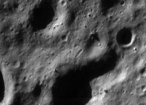
In Fig. 27e was taken during the phase of Chang’e-3 soft landing, from 1 km’s altitude (Jiang et al. 2015). Carefully observe the image it could be found that many different sizes of crater located on this area, however most of them are easily detected because of the contrast between shadow and bright areas. Figure 32 illustrated the landing areas selection, all the connected areas distributed around the craters, the 2th and 14th circular landing area have the maximum in score, and the final landing area is the 2th circular landing area, which is just the target landing area that was selected as described in the reference (Jiang et al. 2015).

Fig. 32

Circular landing areas selection in (e) of Fig. 27. a Connected areas; b areas with the maximum in score; c the final landing area

In Fig. 27f–h were taken by NEAR-Shomaker spacecraft (Veverka et al. 2001)from 433 Eros on February 12, 2001 [NASA PHOTO NEAR image of the day for 2001 Feb 12 (C); NASA PHOTO NEAR image of the day for 2001 Jul 31; NASA PHOTO NEAR image of the day for 2001 Feb 12 (F)], (f) was taken at the height of 250 meters, (g) was taken at the height of about 700 m, and (h) was taken at the height of 120 m. The area in (h) was the final landing area of NEAR-Shomaker spacecraft. From these images we can find that many stones with different sizes distributed in these areas, many of them can be easily detected, the connected areas are all concentrated on the places with no hazard. In Fig. 33, the landing areas with the maximum in score are far from the hazard compare with the others, and the final selected land area is the one with the maximum in radius in these areas. In Fig. 34, the stones with large size concentrated on the edge position of the region in the image, the landing areas with the maximum in score concentrated on the middle position of the region, and the final selected is also the area with the maximum in radius in these landing areas. In Fig. 35, the 3th, 8th and 12th are the landing areas with the maximum in score, expect the 8th area located nearby the huge stone, the other two areas are far from it, and the 3th landing area, which has the maximum in radius is selected as the final landing area.

Fig. 33

Circular landing areas selection in (f) of Fig. 27. a Connected areas; b areas with the maximum in score; c the final landing area

Fig. 34

Circular landing areas selection in (g) of Fig. 27. a Connected areas; b areas with the maximum in score; c the final landing area

Fig. 35

Circular landing areas selection in (h) of Fig. 27. a Connected areas; b areas with the maximum in score; c the final landing area

In Fig. 27, the average time consuming of (a–h) was about 15.6 s, the time consuming was largely depended on the size of image, as we know that the time consuming is crucial, if the time consuming is too long, it will lead to disastrous consequences, so the approach should be simplified to meet the requirement of time limitation.

5 Conclusion

Hazard detection and landing area selection is crucial in the process of asteroid landing, many approaches have been proposed, and some of them had been conducted successfully. However, at present, the avoidance of closed environment (Such as the inner of crater) is not considered in most approaches, for addressing the issue, landing area selection based on closed environment avoidance from a single image during optical coarse hazard detection is proposed in this paper. The approach is designed under the scheme of Chang’e-3′s landing process. It begins with hazard detection based on a proposed binary method. And then, for searching the candidate circular landing areas, the skeletons of areas with no hazard are taken into account, and then, control constraints are considered to select the landing areas that are accessible by the lander. Finally, the final selected circular landing area are chosen by a proposed scoring method, this method combines the factors of circular areas, including circle’s radius, the connection among circular areas, circular area’s texture and the distribution feature of circle’s center to all the hazard. For testing the performance of the approach, experiments were conducted in different kinds of asteroid terrain, from the experiment we can find that the approach can really select a landing area that are not located in the closed environments. However, some issues still needed to be addressed, they can be concluded as followed: First, time consuming of the approach doesn’t meet the requirement of real-time, and the process of the approach is complex, it should be simplified to satisfy engineering requirement. Second, in some cases, the 3D features of landing area cannot be reflected from a single image, an approach of getting 3D features should be addressed.

References

J. Biele, S. Ulamec, Capabilities of Philae, The Rosetta Lander. Origin and Early Evolution of Comet Nuclei (Springer, New York, 2008)
T. Brady, E. Robertson, C. Epp, Hazard detection methods for lunar landing. in Aerospace Conference, 7–14 Mar (2009)
Y. Cheng, A.E. Johnson, L.H. Mattheis et al. Passive imaging based hazard avoidance for spacecraft safe landing, CISSR, 1 Feb (2002)
S.J. Citron, S.E. Dunin, H.F. Meissinger, A terminal guidance technique for lunar landing. Aiaa J. 2(3), 503–509 (2015)
B.J.R. Davidsson, P.J. Gutiérrez, Nucleus properties of Comet 67P/Churyumov–Gerasimenko estimated from non-gravitational force modeling. Icarus 176(2), 453–477 (2005)
A.J.V. Doorn, J.J. Koenderink, Affine structure from motion. J. Opt. Soc. Am. 8(2), 377–385 (1991)
E. Hand, Planetary science. Philae probe makes bumpy touchdown on a comet. Science 346(6212), 900 (2014)
Huertas, Y. Cheng, R. Madison, Passive imaging based multi-cue hazard detection for spacecraft safe landing. in Aerospace Conference, 4–11 Mar (2006)
K. Ikeuchi, B.K.P. Horn et al., Numerical shape from shading and occluding boundaries. Artif. Intell. 59(1), 141–184 (1989)
X. Jiang, T. Tao, S. Li, Innovative hazard detection and avoidance guidance for safe lunar landing. Proc. Inst. Mech. Eng. Part G J. Aerosp. Eng. 230(11), 2086–2103 (2015)
X. Jiang, S. Li, T. Tao, Innovative hazard detection and avoidance strategy for autonomous safe planetary landing. Acta Astronaut. 126, 66–76 (2016)
D.U. Jianping, Z. Han, Optimization model of the trajectory design and control strategies for chang’e-3’s soft-landing. Math. Model. Appl. 3(4), 39-53 (2014) (In Chinese)
A.E. Johnson, A. Huertas, R.A. Werner et al., Analysis of on-board hazard detection and avoidance for safe lunar landing. in Aerospace Conference (IEEE, 2008), pp. 1–9
F. Junhua, C. Pingyuan, C. Hutao, Autonomous hazard detection and landing point selecting for planetary landing. in Systems and Control in Aeronautics and Astronautics, Harbin, 8–10 June (2010)
C. Lantuejoul, in Skeletonization in Quantitative Metallography, ed. by R.M. Haralick, J.C. Simon. Issues in Digital Image Processing (Sijthoff and Noordoff, Amsterdam, 1980), pp. 107–735
Z.Q. Liu, K.C. Di, P. Man et al., High precision landing site mapping and rover localization for Chang’e-3 mission. Sci. China (Phys. Mech. Astron.) 58(1), 1–11 (2015)
L. Matthies, A. Huertas, Y. Cheng et al., Landing hazard detection with stereo vision and shadow analysis. in IEEE International Conference on Robotics and Automation, ICRA 2008, 19–23 May 2008, Pasadena (DBLP, 2008), pp. 2735–2742
D. Meng, C. Yunfeng, W. Qingxian, Method of passive image based crater autonomous detection. Chin. J. Aeronaut. 22(3), 301–306 (2009)
C. Min-Hyun, T. Min-Jea, Reconstruction of high-frequency lunar digital elevation model using shape from shading. INCAS Bull. 10(1), 5–12 (2018)
NASA PHOTO Arabia Terra Crater, https://www.jpl.nasa.gov/spaceimages/details.php?id=PIA22370
NASA PHOTO Hakumyi Crater, https://www.jpl.nasa.gov/spaceimages/details.php?id=PIA21413
NASA PHOTO NEAR image of the day for 2001 Feb 12, http://near.jhuapl.edu/iod/20010212c/index.html
NASA PHOTO NEAR image of the day for 2001 Feb 12 (C), http://near.jhuapl.edu/iod/20010212e/20010212e.tif
NASA PHOTO NEAR image of the day for 2001 Jul 31, http://near.jhuapl.edu/iod/20010731/index.html
NASA PHOTO NEAR image of the day for 2001 Feb 12 (F), http://near.jhuapl.edu/iod/20010212f/20010212f.tif
NASA PHOTO near_20000919_large_anim, https://nssdc.gsfc.nasa.gov/planetary/image/near_20000919_large_anim.gif
NASA PHOTO near_20000511, https://nssdc.gsfc.nasa.gov/planetary/image/near_20000511.jpg
NASA PHOTO Small Craters Peppering South Polar Region, https://www.jpl.nasa.gov/spaceimages/details.php?id=PIA02944
D. Neveu, G. Mercier, J.F. Hamel et al., Passive versus active hazard detection and avoidance systems. Ceas Space J. 7(2), 159–185 (2015)
N.N. Otsu, A threshold selection method from Gray-level. IEEE Trans. Syst. Man Cybern. 9(1), 62–66 (1979)
S.H. Peng, D.H. Kim, S.L. Lee et al., Texture feature extraction based on a uniformity estimation method for local brightness and structure in chest CT images. Comput. Biol. Med. 40(11), 931–942 (2010)
N. Serrano, A Bayesian framework for landing site selection during autonomous spacecraft descent. in IEEE/RSJ International Conference on Intelligent Robots and Systems (IEEE, 2006), pp. 5112–5117
N. Serrano, H. Seraji, Landing site selection using fuzzy rule-based reasoning. in IEEE International Conference on Robotics and Automation, 2007, Roma, 10–14 Apr (2007)
W. Shao, P. Cui, W. Zhou, Safe landing site selection based on computational geometry and genetic algorithm. in Fourth International Conference on Natural Computation (IEEE, 2008), pp. 660–664
S. Ulamec, Landing strategies for small bodies missions.—Philae and beyond. COSPAR Scientific Assembly. DLR, pp. 847–858 (2011)
J. Veverka, B. Farquhar, M. Robinson et al., The landing of the NEAR-Shoemaker spacecraft on asteroid 433 Eros. Nature 413(6854), 390–393 (2001)
Q. Wang, J. Liu, A Chang’E-4 mission concept and Vision of future Chinese lunar exploration activities. Acta Astronaut. 127, 678–683 (2016)
R. Wei, R. Xiaogang, N. Yu et al., Shadow areas robust matching among image sequence in planetary landing. Earth Moon Planets 119(2–3), 95–124 (2017)
H. Xiangyu, C. Hutao, C. Pingyuan, An autonomous optical navigation and guidance for soft landing on asteroids. Acta Astronaut. 54(10), 763–771 (2004)
S. Yamao, M. Miura, S. Sakai et al., A sequential online 3D reconstruction system using dense stereo matching. in Applications of Computer Vision (IEEE, 2015), pp. 341–348
C. Yang, Real-time surface slope estimation by homography alignment for spacecraft safe landing. in IEEE International Conference on Robotics and Automation (IEEE, 2010), pp. 2280–2286
M. Yu, H. Cui, Y. Tian, A new approach based on crater detection and matching for visual navigation in planetary landing. Adv. Space Res. 53(12), 1810–1821 (2014)
C. Zeitlin, D.M. Hassler, F.A. Cucinotta et al., Measurements of energetic particle radiation in transit to Mars on the Mars Science Laboratory. Science 340(6136), 1080–1084 (2013)
Z. Zhang, Determining the epipolar geometry and its uncertainty: a review. Int. J. Comput. Vis. 27(2), 161–195 (1998)
H.H. Zhang, J. Liang, X.Y. Huang et al., Autonomous hazard avoidance control for Chang’E-3 soft landing. Sci. Sinica 44(6), 559 (2014)
Acknowledgements
Hebei natural fund (No. F2018207038); Key Research and Development Program in Hebei (No. 17216108); Hebei Province Applied Basic Research Program (No. 16960314D); Colleges and Universities in Hebei Province Science and Technology Research Project (No. QN2016223); 2016 Hebei University of Economics and Business, Dr. Scientific Research Fund (No. 0112160171); 2016 Hebei University of Economics and Business, Research Fund (No. 2016KYQ01); National Natural Science Foundation of China (No. 61375086).We thank the above mentioned funds for the financial support.
Author information
Authors and Affiliations
Corresponding author
Rights and permissions
About this article
Cite this article
Wei, R., Jiang, J., Ruan, X. et al. Landing Area Selection Based on Closed Environment Avoidance from a Single Image During Optical Coarse Hazard Detection. Earth Moon Planets 121, 73–104 (2018). https://doi.org/10.1007/s11038-018-9516-2
Received:
Accepted:
Published:
Issue Date:
DOI: https://doi.org/10.1007/s11038-018-9516-2