Sequential Rearrangement of Information in Formation of Patterns

Abstract

Beyond their conventional concepts as some outcome of the system dynamics, Patterns and their Formation are regarded here as some substantial parts in description of the dynamics and flow of information in systems. Approach to a typical geometrical problem, for instance, comprises some sequential steps where the observed information (forms and symmetries) of the system is rearranged, reorganized and reformulated to reach the final result. An algebra is introduced here to begin a systematic framework for sequential approaches to geometrical problems. The type of the objects suitable for different kinds of the problems, the way the objects successively match to get a more detailed description of the problem, and the summation operator which combines simultaneous segments of the information of the system are discussed. Based on such abstract clarification for the sequential description of systems, we then switch to reformulate practical examples in various fields from network dynamics to molecular decomposition, relativity and embryogenesis, and demonstrate how different sequential implementation of symmetry could lead to proper description for the dynamics in each of these examples.

Appendices

Appendix 1

1.1 Geometrical Rearrangement

Typical geometric problems are reviewed here where the unknowns are found by rearranging the system information. The rearrangement is such that at each step (i) the original system can be reconstructed from the rearranged system and hence, they are equivalent and (ii) the information are more converged to result the required information.

• (1) Consider a point $O$ inside an equilateral triangle $\Delta ABC$ such that $OA = 4$, $OB = 3$, and $OC = 5$ (Fig. 

  Fig. 27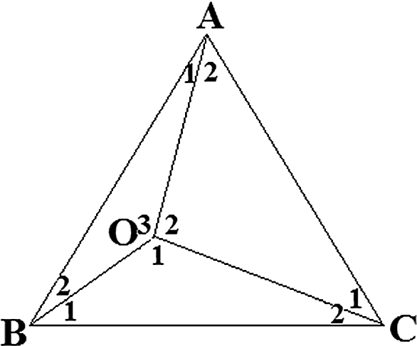

  

  Construction of the problem described by case 1

  27). How much would be $B_{1} + A_{2}$?

The first notice is that with no loss we may dismiss the information of the triangle $\Delta OAB$. Then in order to find the required information ($B_{1} + A_{2}$) the triangles $\Delta OBC$ and $\Delta OAC$ can be reconfigured having $OC$ detached and $AC$ attached to $BC$ as in Fig. 

Fig. 28

Rearrangement of the construction in case 1

28. This results a well-known triangle with sides equal to $3$, $4$ and $5$, and hence, $B_{1} + A_{2} = 90\deg$.

• (2) Consider a point $E$ on the side $AC$ of an equilateral triangle $\Delta ABC$, such that $\angle ABE = 20\deg$ and point $D$ on the side $AB$ such that $\angle ACD = 30\deg$. How much would be $\angle BED$?

The solution is developed by drawing $EG$ parallel to $BC$ and then the segments $CG$ and $DH$ as illustrated by Fig. 

Fig. 29

Construction of the problem described by case 2

29. This actually transforms the information reversibly from $B$ and $C$ to $G$ and $E$ and hence, the information is gathered around the unknown angle $x = \angle BED$. Note that this is a valid rearrangement stage as the original triangle $\Delta ABC$ can be reconstructed by the isosceles triangle $\Delta AGE$ and the equilateral triangle $\Delta GEH$. Also the information of the isosceles triangle $\Delta BDC$ and the equilateral triangle $\Delta BHC$ is transformed to form the isosceles triangle $\Delta BDH$ which gives $\angle DHB = 80\deg$ and hence, $\angle GHD = 40\deg$. So the triangle $\Delta GHD$ is isosceles which combined with $\Delta GEH$ results in $\angle GED = \angle DEH = \angle GEB/2$ and hence, $x = 30\deg$.

Note that the original system can be reconstructed by the triangles $\Delta DGE$ and $\Delta DHE$: $B$ is at the intersection of $EH$ and $DG$ while $A$ is afterwards obtained via the condition $AG = BE$ and finally $C$ is found at the intersection of $AE$ and $BC$ i.e. the passing line on $B$ parallel to $GE$.

Appendix 2

2.1 Representation of Permutation Via Reflection Symmetry

By applying $1 \leftrightarrow 2$ and then $2 \leftrightarrow 3$ one gets the permutation $3,1,2$ while by reversed order of application of these symmetries $2,3,1$ is achieved so as to form a complete permutation set of $1,2,3$. However $2$ is prioritized in such a representation. To remove this or equivalently to emphasize on the fact that there is no priority in applying any of the symmetries $1 \leftrightarrow 2$ and $2 \leftrightarrow 3$, further comment should be added to the sequence. This is the purpose of the symmetry $1 \leftrightarrow 3$. The sequence in this form, therefore, is a complete representation of permutation symmetry via reflection symmetries (Fig. 

Fig. 30

Permutation representation by reflection symmetries

30).

Appendix 3

3.1 Pappus Theorem; Sequences of Lines

Pappus theorem shows another example for a local–global consistent structure i.e. that the consistent definition of conditions in local form gives rise to a representation of the global invariance. Here special correspondence between two sets of collinear points gives rise to a new set of collinear points. Consider three points $A,C,E$ on line $L1$ and $B,D,F$ on $L2$ and that $AB,CD,EF$ intersect with $DE,FA,BC$ respectively at $M,N,L$. These three intersection points are collinear [8]. Typical cases are shown by Fig. 

Fig. 31

Typical constructions of Pappus theorem

31.

Any line can be represented by two points while the points are also to be represented by the intersection of at least two lines. Such conjugacy between the lines and points is depicted in Fig. 

Fig. 32

Line-Point conjugacy in sequential format

32. Converting in sequential format we would write a point as a summation of two lines while each line is shown by a sequence of two points.

Getting back to the description of the Pappus theorem and for the sake of simplicity we utilize a numeric nomination for the points as $1,2,3$ standing for $A,C,E$ and $1^{\prime},2^{\prime},3^{\prime}$ for $B,D,F$:

$$\begin{gathered} AB:[1,1^{\prime}] \equiv [1^{\prime},1] \hfill \\ ED:[3,2^{\prime}] \equiv [2^{\prime},3] \hfill \\ \end{gathered}$$

(30)

and for their intersection point:

$$M:AB + ED \equiv [3,2^{\prime}] + [1,1^{\prime}]$$

(31)

Similarly we get:

$$\begin{gathered} N:[1,3^{\prime}] + [2,2^{\prime}] \hfill \\ L:[2,1^{\prime}] + [3,3^{\prime}] \hfill \\ \end{gathered}$$

(32)

Using (31) and (32) the lines $MN$ and $ML$ are shown as:

$$\begin{gathered} MN:[[3,2^{\prime}] + [1,1^{\prime}]],[[1,3^{\prime}] + [2,2^{\prime}]] \hfill \\ ML:[[3,2^{\prime}] + [1,1^{\prime}]],[[2,1^{\prime}] + [3,3^{\prime}]] \hfill \\ \end{gathered}$$

(33)

This gives the following for their intersection:

$$([[3,2^{\prime}] + [1,1^{\prime}]],[[1,3^{\prime}] + [2,2^{\prime}]]) + ([[3,2^{\prime}] + [1,1^{\prime}]],[[2,1^{\prime}] + [3,3^{\prime}]])$$

(34)

equal to:

$$\left[ \mathop{\updownarrow}^{3}_{1} ,\; \mathop{\updownarrow}_{1^{\prime}}^{2^{\prime}} \right],\;\left[ \mathop{\updownarrow}^{1}_{2} ,\; \mathop{\updownarrow}^{3^{\prime}}_{2^{\prime}} \right]\; + \;\left[ \mathop{\updownarrow}^{3}_{1} ,\; \mathop{\updownarrow}^{2^{\prime}}_{1^{\prime}} \right],\;\left[ \mathop{\updownarrow}^{2}_{3} ,\; \mathop{\updownarrow}^{1^{\prime}}_{3^{\prime}} ,\right]$$

(35)

Fig. 33

Summation action on Pappus sequences

Figure 33 shows that such a sequence involves representations of permutations in $1,2,3$ and $1^{\prime},2^{\prime},3^{\prime}$ (see “Appendix 2”; the permutation representation via reflection symmetry).

By applying the permutation $1,2,3 \to 2,3,1$ and $1^{\prime},2^{\prime},3^{\prime} \to 2^{\prime},3^{\prime},1^{\prime}$ there is no change in the description of the problem:

$$([[1,3^{\prime}] + [2,2^{\prime}]],[[2,1^{\prime}] + [3,3^{\prime}]]) + ([[1,3^{\prime}] + [2,2^{\prime}]],[[3,2^{\prime}] + [1,1^{\prime}]])$$

(36)

which is equivalent to the intersection of the lines $MN$ and $LN$. Together with (34) this emphasizes that:

$$MN + ML \equiv MN + LN$$

(37)

which means that the points $M,N,L$ are three points on the same line. Another fruitfulness of the sequential representation for the Pappus theorem is that by looking for other admissible forms we directly reach at variations of the problem which could be found via changing the intersections. These variations correspond to different combination of the indices in representations of the form (36). Any change of a combination is admissible provided that tensor summation notation is followed i.e. that at each of the two subsequences (added to form the whole sequence) the repetitive numbers appear in different rows (one at the upper and one the lower row). One variation of the form (36), for instance, can be found as:

$$\left[ \mathop{\updownarrow}^{2}_{3} ,\; \mathop{\updownarrow}_{1^{\prime}}^{2^{\prime}} \right],\;\left[ \mathop{\updownarrow}^{3}_{1} ,\; \mathop{\updownarrow}^{3^{\prime}}_{2^{\prime}} \right]\; + \;\left[ \mathop{\updownarrow}^{2}_{3} ,\; \mathop{\updownarrow}^{2^{\prime}}_{1^{\prime}} \right],\;\left[ \mathop{\updownarrow}^{1}_{2} ,\; \mathop{\updownarrow}^{1^{\prime}}_{3^{\prime}} ,\right]$$

(38)

which corresponds to:

$$([[2,2^{\prime}] + [3,1^{\prime}]],[[3,3^{\prime}] + [1,2^{\prime}]]) + ([[2,2^{\prime}] + [3,1^{\prime}]],[[1,1^{\prime}] + [2,3^{\prime}]])$$

(39)

This version of the problem is shown by Fig. 

Fig. 34

Typical version of Pappus construction

34.

Appendix 4

4.1 Convergence to the Symmetric Pattern in Morley’s Variants

4.1.1 Local Reflection Consistent with Global Permutation

As for the first perturbation of the Morley’s construction we merely preserve the local reflection symmetry i.e. $A_{1} = A_{3} = kA$, $B_{1} = B_{3} = kB$, $C_{1} = C_{3} = kC$ where $k$ is not necessarily equal to $1/3$ as discussed in Sect. 2.4. The ratio of the maximum side length to the minimum one in the semi-equilateral triangle produced after two iterations of such perturbed Morley’s construction is shown in Fig. 

Fig. 35

The ratio of the maximum-to-minimum sides in the semi-equilateral triangle produced after 2 iterations of the $40\%$ perturbed Morley’s procedure. The starting triangles varies in $A$ and $B$ from $20$ to $60$ and $20$ to $90\deg$ respectively

35 for $k = 0.2$ (corresponding to the nominal perturbation size $p = (1 - 3k) = ((1 - 2k)A - kA)/A$ equal to $40\%$) for a wide range of $A$ and $B$ values. Dissimilarity to perfect equilateral triangle is below $1.2\%$. For $k = 0.1$ ($70\%$ perturbation) dissimilarity is below $3.5\%$ as shown by Fig. 

Fig. 36

The ratio of the maximum-to-minimum sides in the semi-equilateral triangle produced after 2 iterations of the $70\%$ perturbed Morley’s procedure. The starting triangles varies in $A$ and $B$ from $20$ to $60$ and $20$ to $90\deg$ respectively

36. The following code corresponds to the above procedure. The angular outputs of the code should be used as the inputs for the next iteration.

function [E,F,G] = ExtendedMorley( A, B).

A = A*pi/180;

B = B*pi/180;

C = pi - A - B;

k = 0.1;

AG = sin(C)*sin(k*B)/sin(k*(A + B));

BG = sin(C)*sin(k*A)/sin(k*(A + B));

AF = sin(B)*sin(k*C)/sin(k*(A + C));

CF = sin(B)*sin(k*A)/sin(k*(A + C));

CE = sin(A)*sin(k*B)/sin(k*(B + C));

BE = sin(A)*sin(k*C)/sin(k*(B + C));

GF = sqrt(AG^2 + AF^2 - 2*AG*AF*cos((1–2*k)*A));

FE = sqrt(CF^2 + CE^2 - 2*CF*CE*cos((1–2*k)*C));

EG = sqrt(BG^2 + BE^2 - 2*BG*BE*cos((1–2*k)*B));

E = (180/pi)*acos((FE^2 + EG^2 - GF^2)/(2*FE*EG));

F = (180/pi)*acos((FE^2 + GF^2 - EG^2)/(2*FE*GF));

G = (180/pi)*acos((GF^2 + EG^2 - FE^2)/(2*GF*EG));

4.1.2 Local Reflection Inconsistent with Global Permutation

For such variation we keep reflections locally but these symmetries are not to be consistent with the global permutation i.e. we drop the symmetries $A_{13} \leftrightarrow B_{13}$, (which means the reflection $A_{1} \leftrightarrow A_{3}$ does not admit $B_{1} \leftrightarrow B_{3}$), $B_{13} \leftrightarrow C_{13}$, and $C_{13} \leftrightarrow A_{13}$. By such constructions no permutation is achieved via the summations of the form (15) and hence, no symmetric pattern would be expected. A typical case could be $A_{1} = A_{3} = 0.5(1 - A/\pi )A,A_{2} = (A/\pi )A$, $B_{1} = B_{3} = 0.5(1 - B/\pi )B,B_{2} = (B/\pi )B$, and $C_{1} = C_{3} = 0.5(1 - C/\pi )C,C_{2} = (C/\pi )C$. Figure 

Fig. 37

The ratio of the maximum-to-minimum sides in the triangle produced after 2 iterations of the Morley’s procedure; variant (ii). The starting triangles varies in $A$ and $B$ from $20$ to $60$ and $20$ to $90\deg$ respectively

37 shows that after 2 iterations the system final pattern diverges from equilateral by more than $100\%$ (the maximum-to minimum ratio is greater than 2) except for the trivial case where the initial triangle is an equilateral one.

4.1.3 Local Permutation Consistent with Global Permutation

Finally we drop local reflections completely but there still should be a local permutation consistent with global i.e. the permutations $A_{1} \to A_{2} \to A_{3}$, $B_{1} \to B_{2} \to B_{3}$, and $C_{1} \to C_{2} \to C_{3}$ admit each other. Generally this is equivalent to $A_{1} = k_{1} A,$ $A_{2} = k_{2} A,$ $A_{3} = (1 - k_{1} - k_{2} )A$, $B_{1} = k_{1} B,$ $B_{2} = k_{2} B,$ $B_{3} = (1 - k_{1} - k_{2} )B$, and $C_{1} = k_{1} C,$ $C_{2} = k_{2} C,$ $C_{3} = (1 - k_{1} - k_{2} )C$. Figure 

Fig. 38

The ratio of the maximum-to-minimum sides in the triangle produced after 20 iterations of the Morley’s procedure; variant (iii). The starting triangles varies in $A$ and $B$ from $20$ to $60$ and $20$ to $90\deg$ respectively

38 shows that for a typical case $k_{1} = 0.7,k_{2} = 0.2$ the dissimilarity of the system’s final pattern to a perfect equilateral is less than $5\%$. This, however, occurs after 20 iterations which implies a much slower convergence rate compared to the local–global reflection scenario (i).

Appendix 5

5.1 Binary-Phase Decomposition Modified with External Loading

For decomposition on an elastic surface (half space) the modified Cahn–Hilliard model reads [18, 19]:

$$\frac{\partial C}{{\partial t}} = \alpha \nabla^{2} \left(\frac{\partial g}{{\partial C}} - \beta \nabla^{2} C + \varphi_{\alpha \beta } \varepsilon_{\alpha \beta }^{m} + \varphi_{\alpha \beta } \varepsilon_{\alpha \beta }^{e} \right).$$

(40)

$\varepsilon_{\alpha \beta }^{m}$ is a passive strain accompanying the self-assembly process that resists the relaxation of the monolayer, while $\varepsilon_{\alpha \beta }^{e}$ is an active strain due to the external loading. $\varphi_{\alpha \beta }$ relates the surface stress to the concentration. For $\varphi_{11} = \varphi_{22} = \varphi$ and $\varphi_{12} = \varphi_{21} = 0$ the dilatation enters the Eq. (40) which comprises two parts. The first part is due to the action of the concentration dependent surface stress (of the binary mixture) on an isotropic half space (substrate). This problem is solved by superposition of the Cerruti’s solution of a point force on a half space:

$$\varepsilon_{\beta \beta }^{m} = - \frac{{(1 - \nu^{2} )\varphi }}{\pi E}\iint {\frac{{(x - \xi_{1} )\frac{\partial C}{{\partial \xi_{1} }} + (y - \xi_{2} )\frac{\partial C}{{\partial \xi_{2} }}}}{{[(x - \xi_{1} )^{2} + (y - \xi_{2} )^{2} ]^{3/2} }}}d\xi_{1} d\xi_{2}.$$

(41)

The second part $\varepsilon_{\beta \beta }^{e}$ is due to an external loading which can be used to control the pattern formation of the original system. The Eq. (41) in non-dimensional form reads [18, 19]:

$$\frac{\partial C}{{\partial t}} = \nabla^{2} (P(C) - 2\nabla^{2} C - \frac{Q}{\pi }\iint {\frac{{(x - \xi_{1} )\frac{\partial C}{{\partial \xi_{1} }} + (y - \xi_{2} )\frac{\partial C}{{\partial \xi_{2} }}}}{{[(x - \xi_{1} )^{2} + (y - \xi_{2} )^{2} ]^{3/2} }}}d\xi_{1} d\xi_{2} + \hat{R})$$

(42)

$P(C)$ is taken as $\ln (C/(1 - C)) + 2.2(1 - 2C)$ where with the average concentration $mean(C) = C_{0} = 0.5$ in this system $C > 0.5$ indicates the dominance of the component $A$ and $C < 0.5$ dominance of $B$. $Q$ is the ratio of two characteristic length scales of the system and is set to be $1$ and $\hat{R}$ is a dimensionless parameter measuring the strength of external loading (strain) defined as:

$$\hat{R} = \varphi_{\alpha \beta } \varepsilon_{\alpha \beta }^{e} /(\Lambda k_{b} T),$$

(43)

where $\Lambda$ is the number of atoms per unit area on the surface, $k_{b}$ is the Boltzmann’s constant, and $T$ is the absolute temperature [18, 19]. Taking Fourier transform of (42) one gets:

$$\frac{\partial FC}{{\partial t}} = - \omega^{2} FP - 2\omega^{4} FC + 2\omega^{3} FC + F\hat{R}$$

(44)

after which numerical solution using a semi-implicit approach can be pursued [9, 18]. Simulation result for a squared shape loading (Fig. 

Fig. 39

External loading (dilatation) on system (42), $\hat{R} = 0$ in black and $\hat{R} = 1$ in white

39) is shown in Fig. 

Fig. 40

Simulation result due to the external loading shown in Fig. 39 at $1000$ time steps

40. The symmetry in this case is applied locally to the edges and the roll formation slowly starts in the neighborhood of the edges since each symmetry generator at the vicinity of its corresponding edges has priority to the other.

Appendix 6

6.1 Stiffness Directed Differentiation in Circular Domain

A combined elasticity/relocation model explains how the stem cells could measure different values for the stiffness of their surroundings [12]. In response to such a variety of the experienced stiffnesses different tissue formations trigger which facilitate the constitution of an entire organ [12]. For a circular domain which resembles the cross section of a typical limb, for instance, the cells relocate towards the center (Fig. 

Fig. 41

Changes in the cell density across a limb cross section (a), the modified stiffness (b) and formation of a bone collar at the cartilage-muscle boundary (c). Changes in the cell density across an enlarged domain (d), the modified stiffness (e) and the emergence of a soft tissue inside the bone collar (f)

41a). Therefore due to the lower intracellular distances in higher congestions, the experienced stiffness in a central disk is higher compared to peripheral domains and this suggests the central cartilage formation in a limb. The experienced stiffness, however, is modified due to a secondary effect caused by the Extra Cellular Matrix (ECM) deformation. The resultant stiffness is highest within a ring (Fig. 41b) which leads to formation of a bone collar (Fig. 41c). The internal region to such a ring experiences the intermediate stiffness range corresponding to the cartilage formation (eventually transformed into the bone marrow) while at the external region the stiffness is in the softest range corresponding to muscular and vascular formation.

By enlarging the domain the modification effect of the ECM improves (Fig. 41d and e) which makes the experienced stiffness at the internal (the former cartilage) domain to fall as down as to the soft tissue limit. Therefore actually a bifurcation takes place by emergence of a soft tissue domain inside the hard tissue (Fig. 41f).

References

Murray, J.D.: Mathematical biology, II: Spatial models and biomedical applications, 3rd edn. Springer, New York (2003)
Nelson, C.M.: Geometric control of morphogenesis. Biochim. Biophys. Acta (2009). https://doi.org/10.1016/j.bbamcr.2008.12.014
Jörg, D., Oates, A.C., Jülicher, F.: Sequential pattern formation governed by signaling gradients. Phys. Biol. (2016). https://doi.org/10.1088/1478-3975/13/5/05LT03
Geitmann, A., Ortega, J.K.E.: Mechanics and modeling of plant cell growth. Trends Plant Sci. (2009). https://doi.org/10.1016/j.tplants.2009.07.006
Boudaoud, A.: An introduction to the mechanics of morphogenesis for plant biologists. Trends Plant Sci. (2010). https://doi.org/10.1016/j.tplants.2010.04.002
Meinhardt, H., Koch, A.J., Bernasconi, G.: Models of pattern formation applied to plant development. Symmetry Plants (1998). https://doi.org/10.1142/9789814261074_0027
Haji, A.H.: Sequence, symmetry and pattern formation. Math. Comput. Model (2010). https://doi.org/10.1016/j.mcm.2010.06.029
Coxeter, H.S.M., Greitzer, S.L.: Geometry revisited. Random House Inc., New York (1967)
Haji, A.H., Mahzoon, M., Javadpour, S.: Pattern formation and geometry of the manifold. Commun. Nonlinear Sci. Numer. Simul. (2011). https://doi.org/10.1016/j.cnsns.2010.06.019
Guan, S., Lai, C.-H., Wei, G.W.: Geometry and boundary control of pattern formation and competition. Physica D (2003). https://doi.org/10.1016/S0167-2789(02)00737-6
Hoyle, R.: Pattern formation, an introduction to methods. Cambridge University Press, Cambridge (2006)
Haji, A.H.: Mechanical explanation for simultaneous formation of different tissues in an organ morphogenesis. Acta Mech. (2020). https://doi.org/10.1007/s00707-020-02693-9
Martini, F.H., Timmons, M.J., Tallitsch, R.B.: Human anatomy, 7th edn. Pearson Education Inc., London (2012)
McGrew, M.J., Pourquié, O.: Somitogenesis; segmenting a vertebrate. Curr. Opin. Genet. Dev. (1998). https://doi.org/10.1016/S0959-437X(98)80122-6
Baker, R.E., Schnell, S., Maini, P.K.: A clock and wavefront mechanism for somite formation. Dev. Biol. (2006). https://doi.org/10.1016/j.ydbio.2006.01.018
Maini, P.K., Baker, R.E., Schnell, S.: Rethinking models of pattern formation in somitogenesis. Cell Syst. (2015). https://doi.org/10.1016/j.cels.2015.10.004
Naganathan, S.R., Oates, A.C.: Patterning and mechanics of somite boundaries in zebrafish embryos. Semin. Cell Dev. Biol. (2020). https://doi.org/10.1016/j.semcdb.2020.04.014
Lu, W., Suo, Z.: Dynamics of nanoscale pattern formation of an epitaxial monolayer. J. Mech. Phys. Solids (2001). https://doi.org/10.1016/S0022-5096(01)00023-0
Lu, W., Kim, D.: Engineering nanophase self—assembly with elastic field. Acta Mater. (2005). https://doi.org/10.1016/j.actamat.2005.04.021
Author information
Authors and Affiliations
Corresponding author
Ethics declarations
Conflict of interest
The author declares that he has no conflict of interest.
Additional information
Publisher's Note
Springer Nature remains neutral with regard to jurisdictional claims in published maps and institutional affiliations.